
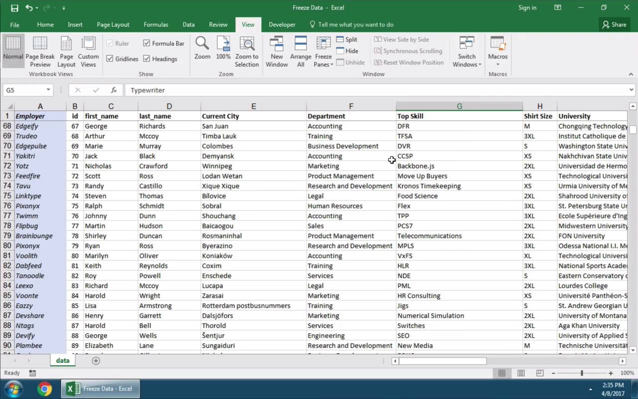
Freeze panes to lock rows and columns
To keep an area of a worksheet visible while you scroll to another area of the worksheet, go to the View tab, where you can Freeze Panes to lock specific rows and columns in place, or you can Split panes to create separate windows of the same worksheet.

Freeze rows or columns
Freeze the first column
-
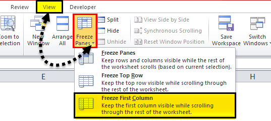
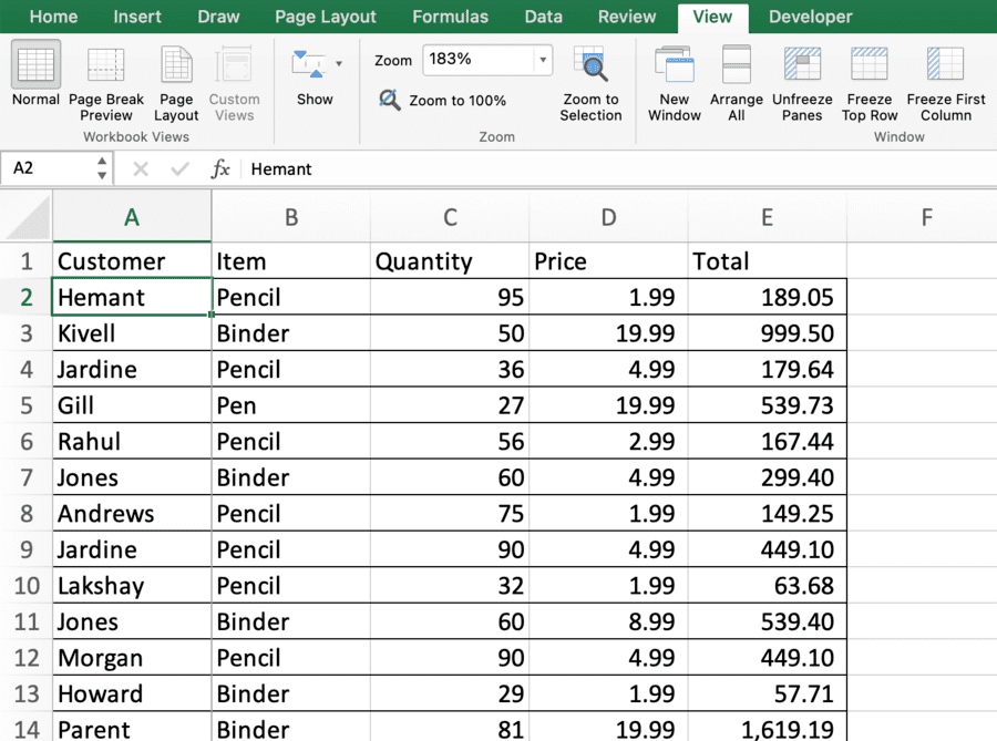
Select View > Freeze Panes > Freeze First Column.
The faint line that appears between Column A and B shows that the first column is frozen.
Freeze the first two columns
-
Select the third column.
-
Select View > Freeze Panes > Freeze Panes.
Freeze columns and rows
-
Select the cell below the rows and to the right of the columns you want to keep visible when you scroll.
-
Select View > Freeze Panes > Freeze Panes.
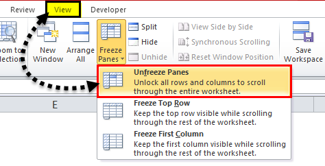
Unfreeze rows or columns
-
On the View tab > Window > Unfreeze Panes.

Note: If you don’t see the View tab, it’s likely that you are using Excel Starter. Not all features are supported in Excel Starter.

Need more help?
You can always ask an expert in the Excel Tech Community or get support in the Answers community.
See Also
Freeze panes to lock the first row or column in Excel 2016 for Mac
Split panes to lock rows or columns in separate worksheet areas
Overview of formulas in Excel
How to avoid broken formulas
Find and correct errors in formulas
Keyboard shortcuts in Excel
Excel functions (alphabetical)
Excel functions (by category)
Need more help?
Freeze Top Row | Unfreeze Panes | Freeze First Column | Freeze Rows | Freeze Columns | Freeze Cells | Magic Freeze Button
If you have a large table of data in Excel, it can be useful to freeze rows or columns. This way you can keep rows or columns visible while scrolling through the rest of the worksheet.
Freeze Top Row
To freeze the top row, execute the following steps.
1. On the View tab, in the Window group, click Freeze Panes.

2. Click Freeze Top Row.

3. Scroll down to the rest of the worksheet.
Result. Excel automatically adds a dark grey horizontal line to indicate that the top row is frozen.

Unfreeze Panes
To unlock all rows and columns, execute the following steps.
1. On the View tab, in the Window group, click Freeze Panes.
2. Click Unfreeze Panes.

Freeze First Column
To freeze the first column, execute the following steps.
1. On the View tab, in the Window group, click Freeze Panes.
2. Click Freeze First Column.

3. Scroll to the right of the worksheet.
Result. Excel automatically adds a dark grey vertical line to indicate that the first column is frozen.

Freeze Rows
To freeze rows, execute the following steps.
1. For example, select row 4.
2. On the View tab, in the Window group, click Freeze Panes.
3. Click Freeze Panes.

4. Scroll down to the rest of the worksheet.
Result. All rows above row 4 are frozen. Excel automatically adds a dark grey horizontal line to indicate that the first three rows are frozen.

Freeze Columns
To freeze columns, execute the following steps.
1. For example, select column E.
2. On the View tab, in the Window group, click Freeze Panes.
3. Click Freeze Panes.
4. Scroll to the right of the worksheet.
Result. All columns to the left of column E are frozen. Excel automatically adds a dark grey vertical line to indicate that the first four columns are frozen.

Freeze Cells
To freeze cells, execute the following steps.
1. For example, select cell C3.
2. On the View tab, in the Window group, click Freeze Panes.
3. Click Freeze Panes.
4. Scroll down and to the right.
Result. The orange region above row 3 and to the left of column C is frozen.

Magic Freeze Button
Add the magic Freeze button to the Quick Access Toolbar to freeze the top row, the first column, rows, columns or cells with a single click.
1. Click the down arrow.
2. Click More Commands.

3. Under Choose commands from, select Commands Not in the Ribbon.
4. Select Freeze Panes and click Add.

5. Click OK.
6. To freeze the top row, select row 2 and click the magic Freeze button.

7. Scroll down to the rest of the worksheet.
Result. Excel automatically adds a dark grey horizontal line to indicate that the top row is frozen.

Note: to unlock all rows and columns, click the Freeze button again. To freeze the first 4 columns, select column E (the fifth column) and click the magic Freeze button, etc.
Freezing panes in excel helps freeze one or more rows and/or columns so that they remain fixed while scrolling through the database. Freezing panes is helpful when the dataset is large and there is a need to view certain sections of the data at all times.
For example, to freeze the first three rows and the first three columns of a blank Excel worksheet, we undertake the following steps:
- Select the cell D4.
- Click the “freeze panes” drop-down from the View tab of the Excel ribbon.
- Select the option “freeze panes.”
Rows 1, 2, and 3 and columns A, B, and C are frozen. Hence, by freezing panes, the user knows the kind of data contained in these fixed rows (1, 2, and 3) and columns (A, B, and C). Moreover, since these rows and columnsA cell is the intersection of rows and columns. Rows and columns make the software that is called excel. The area of excel worksheet is divided into rows and columns and at any point in time, if we want to refer a particular location of this area, we need to refer a cell.read more can be viewed at any point of time, one need not go back to them again and again.
Likewise, freezing excel panes can be applied to the row and column headers of a database. This allows one to constantly view the headings.
With the “freeze panes” drop-down (in the View tab), one can freeze any of the following areas of a worksheet:
- The first row or the first column
- The panes, which includes:
- one or more rows beginning from the top and/or
- one or more columns beginning from the left
Let us consider some examples to understand the working of freezing panes in Excel.
Table of contents
- Freeze Panes in Excel
- Freeze Panes in Excel Examples
- Example #1–Freeze the Top Row in Excel
- Example #2–Freeze the First Column in Excel
- Example #3–Freeze the Top Row and the First Column Together
- Freeze Multiple Rows and Columns Together in Excel
- Shortcut to Freeze Panes in Excel
- Unfreeze Panes in Excel
- The Purpose of Freezing Panes in Excel
- Frequently Asked Questions
- Recommended Articles
- Freeze Panes in Excel Examples
Freeze Panes in Excel Examples
You can download this Freeze Pans Excel Template here – Freeze Pans Excel Template
Example #1–Freeze the Top Row in Excel
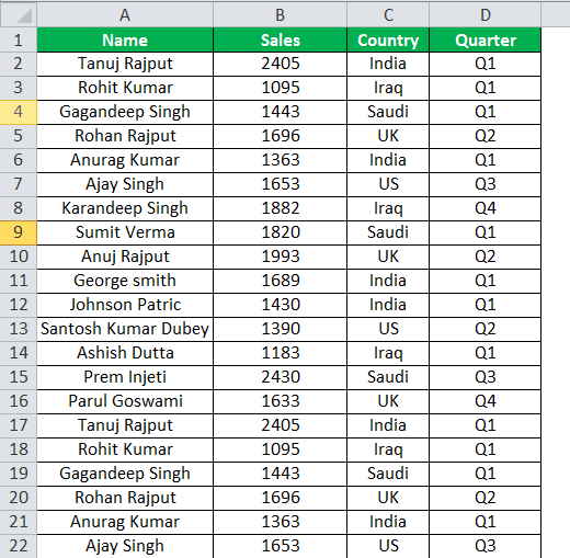
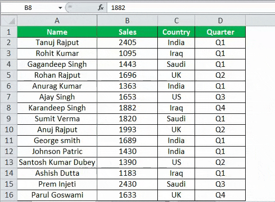
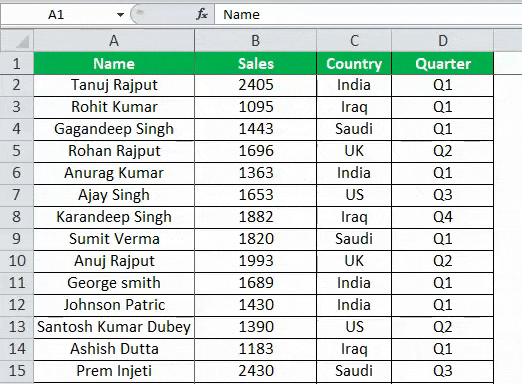
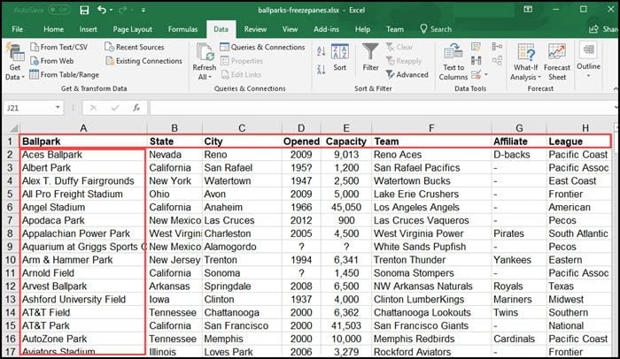
The following image shows the sales revenueSales revenue refers to the income generated by any business entity by selling its goods or providing its services during the normal course of its operations. It is reported annually, quarterly or monthly as the case may be in the business entity’s income statement/profit & loss account.read more (in $ in column B) generated in various countries (column C) by the different sales personnel (column A) of an organization. The entire data relates to the four quarters of a year.
We want to freeze the top row (row 1) of the given dataset.
The steps for freezing the first row in Excel are listed as follows:
- Click the “freeze panes” drop-down from the “window” group of the View tab. Select “freeze top row” as shown in the following image.

- The entire first row (row 1) is frozen. A horizontal gray line appears right below row 1. This line indicates that the row immediately above is frozen.
To cross-check, one can scroll down the worksheet. The row containing the column headers is fixed. The same is shown in the following image.

Example #2–Freeze the First Column in Excel
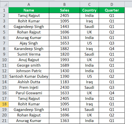
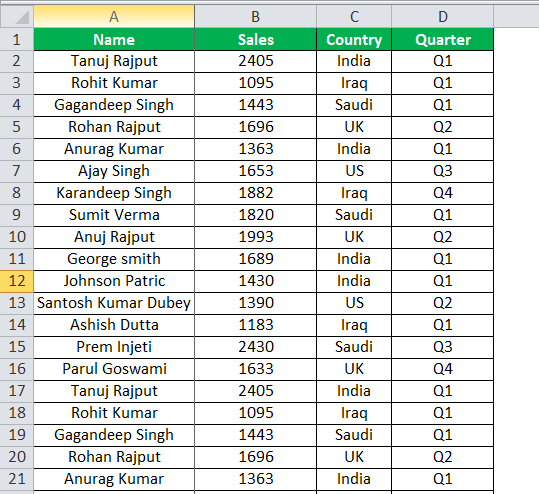
Working on the data of example #1, we want to freeze the first column (column A) of the given dataset.
The steps for freezing the first column of Excel are listed as follows:
Step 1: From the “window” group of the View tab, click the “freeze panes” drop-down. Select “freeze first column,” as shown in the following image.
Step 2: The entire first column (column A) is frozen. A vertical gray line appears right next to column A (or between columns A and B). This line indicates that the column immediately to the left is frozen.
If one scrolls from left to right, column A stays at its place. The same is shown in the following image.
Example #3–Freeze the Top Row and the First Column Together
Working on the data of example #1, we want to freeze the first row (row 1) and the first column (column A) simultaneously.
The steps to freeze the first row and the first column simultaneously are listed as follows:
Step 1: Select the cell B2. From the “freeze panes” drop-down (in the View tab), select “freeze panes.” The same is shown in the following image.

Step 2: Row 1 and column A, both are frozen. A horizontal grey line appears below row 1 and a vertical grey line appears right next to column A. The same is shown in the following image.
The row immediately preceding the active cell (B2) is frozen. Likewise, the column immediately to the left of cell B2 is also frozen.
Note: One must select the cell (in step 1) cautiously. This is because the “freeze panes” option works on the basis of the current selection. It freezes the rows and columns immediately preceding the active or the selected cell.
Freeze Multiple Rows and Columns Together in Excel
The steps to freeze multiple rows and columns are listed as follows:
Step 1: Select the correct cell. The selected cell should be positioned as follows:
- a. The selected cell should be immediately below the last row to be frozen.
- b. The selected cell should be to the immediate right of the last column to be frozen.
Follow both the pointers a and b to freeze multiple rows and columns simultaneously.
Step 2: Select “freeze panes” from the “freeze panes” drop-down of the View tab.
The rows and columns immediately preceding the selected cell (selected in step 1) are frozen.
Note: It is also possible to freeze either multiple rows or multiple columns. One can freeze as many rows and/or columns as one wants. However, the freezing of multiple rows and/or columns should begin from the first row (row 1) and the first column (column A) respectively.
Shortcut to Freeze Panes in Excel
The shortcuts to freeze panes in excel are mentioned as follows:
- To freeze rows and columns both: Press the keys “Alt+W+F+F” one by one. This freezes rows and columns preceding the currently selected cell.
- To freeze the top row only: Press the keys “Alt+W+F+R” one by one. This freezes the first row (row 1) of the worksheet irrespective of the currently selected cell.
- To freeze the leftmost column only: Press the keys “Alt+W+F+C” one by one. This freezes the first column (column A) of the worksheet irrespective of the currently selected cell.
Unfreeze Panes in Excel
The steps to unfreeze panes in excel are listed as follows:
Step 1: Click the drop-down arrow of “freeze panes” in the “window” group of the View tab.
Step 2: Click “unfreeze panes,” as shown in the succeeding image. The gray lines, which appeared as a result of freezing, will disappear.
The “unfreeze panes” option is quite useful when one is unable to figure out where the freezes have been applied in the worksheet.
Note 1: The “unfreeze panes” option appears (under the drop-down of “freeze panes”) after one or more rows and/or columns are frozen by the user.
Note 2: Once the “unfreeze panes” option is clicked, the rows and columns are no longer fixed. So, the worksheet prior to freezing is displayed.
The Purpose of Freezing Panes in Excel
The objectives of freezing panes in excel are listed as follows:
- To prevent referring to the same set of data repeatedly, thus saving the scrolling time of the user
- To know which row or column represents which data
- To facilitate comparisons of the different sections of the worksheet
Frequently Asked Questions
1. What does freezing panes mean and where is this option in Excel?
Freezing panes helps lock or fix certain rows and/or columns of a worksheet so that they remain stationary with a movement through the database. For instance, while working with large datasets, the user may need to keep the row or column headers visible at all times.
By freezing panes, the scrolling time of the user is reduced. This is because the need to refer to the same worksheet area repeatedly is eliminated. Moreover, making comparisons between the different rows or columns becomes easier.
The “freeze panes” option is available under the “freeze panes” drop-down (in the “window” group) of the View tab of Excel. This option freezes one or more rows and/or columns based on the current selection.
In addition, one can use the options “freeze top row” and “freeze first column” (under the “freeze panes” drop-down) to freeze the first row and the first column respectively.
2. How to freeze panes horizontally and vertically in Excel?
To freeze panes horizontally, the user needs to freeze one or more rows. To freeze panes vertically, one or more columns need to be frozen.
The steps to freeze one or more rows and/or columns are listed as follows:
a. Select the relevant cell. This cell should be immediately below the last row to be frozen. Further, it should be to the right of the last column to be frozen.
b. From the “freeze panes” drop-down (in the “window”d group) of the View tab, select “freeze panes”.
The row preceding the active cell (selected in step a) is frozen. Moreover, the column to the left of this cell is also frozen. The gray lines appear which indicate the frozen panes.
Note: With this method, one can freeze any number of rows and columns. The condition is that the freezing of panes must begin from the first row (row 1) and the first column (column A). In other words, the rows and columns in the middle of the worksheet cannot be frozen.
3. How to freeze multiple panes in Excel?
It is possible to freeze multiple rows and columns simultaneously in Excel. However, one cannot freeze panes in the middle of the worksheet. For instance, one cannot create a horizontal pane consisting of rows 9, 10, and 11.
The user can create a horizontal pane which consists of stationary rows beginning from row 1. Likewise, a vertical pane consisting of stationary columns, beginning from column A, can be created.
Apart from one horizontal pane and one vertical pane, it is not possible to create additional panes in the middle of the worksheet. Hence, one cannot create multiple horizontal or multiple vertical panes in Excel.
In other words, a horizontal pane (rows 1, 2, and 3) followed by a scrollable area (rows 4, 5, and 6), and again a horizontal pane (rows 7, 8, and 9) cannot be created.
Recommended Articles
This has been a guide to freezing panes in Excel. Here we discuss how to freeze the rows and columns in Excel by using the “freeze panes” option. We also went through some examples. You can download an Excel template from the website. You may also look at these useful functions of Excel–
- Freeze Excel CellFreezing cells in excel is when we move up or down in the sheet, we freeze desired cells, not to be moved. To freeze cells in excel, select the cells to freeze. Then, in the View tab of the windows section, click on freeze panes.read more
- Freeze Columns in ExcelFreezing columns in excel fixes or locks them so that they remain visible while scrolling through the database. A frozen column does not move with the movement of the remaining columns.read more
- Insert Multiple Excel Rows
- How to Unhiding Columns in Excel?
![]()
Download Article
![]()
Download Article
When you freeze a column or a row, it will stay visible when you’re scrolling through that worksheet, which is a useful tool when you’re comparing data. When you freeze columns or rows, they are referred to as «panes.» This wikiHow will show you how to freeze and unfreeze panes to lock rows and columns in Excel.
-
1
Open your project in Excel. You can either open the program within Excel by clicking File > Open, or you can right-click the file in your file explorer.
- This will work for Windows and Macs using Excel for Office 365, Excel for the web, Excel 2019, Excel 2016, Excel 2013, Excel 2010, Excel 2007.[1]
- This will work for Windows and Macs using Excel for Office 365, Excel for the web, Excel 2019, Excel 2016, Excel 2013, Excel 2010, Excel 2007.[1]
-
2
Select a cell to the right of the column you want to freeze. The frozen columns will remain visible when you scroll through the worksheet.
- You can press Ctrl or Cmd as you click a cell to select more than one, or you can freeze each column individually.
Advertisement
-
3
Click View. You’ll see this either in the editing ribbon above the document space or at the top of your screen.
-
4
Click Freeze Panes. A menu will drop-down.
-
5
Click Freeze Panes. This will freeze the panes in the columns next to what you have selected.[2]
- You’ll notice when you freeze panes if you scroll away and a column or row stays on the screen.


Advertisement
-
1
Open your project in Excel. You can either open the program within Excel by clicking File > Open, or you can right-click the file in your file explorer.
- This will work for Windows and Macs using Excel for Office 365, Excel for the web, Excel 2019, Excel 2016, Excel 2013, Excel 2010, Excel 2007.[3]
- This will work for Windows and Macs using Excel for Office 365, Excel for the web, Excel 2019, Excel 2016, Excel 2013, Excel 2010, Excel 2007.[3]
-
2
Select a cell to the right of the column you want to freeze. The frozen columns will remain visible when you scroll through the worksheet.
-
3
Press the Ctrl or ⌘ Cmd key as you click. All the cells you click will be added to your selection when you have that key pressed.
- You can release the key when you are done making your selections.
-
4
Click View. You’ll see this either in the editing ribbon above the document space or at the top of your screen.
-
5
Click Freeze Panes. A menu will dropdown.
-
6
Click Freeze Panes. This will freeze the panes in the columns next to what you have selected.[4]
- You’ll notice when you freeze panes if you scroll away and a column or row stays on the screen.


Advertisement
-
1
Open your project in Excel. You can either open the program within Excel by clicking File > Open, or you can right-click the file in your file explorer.
-
2
Go to View. You’ll see a drop-down menu.
-
3
Click Freeze Panes. It’s next to Arrange All and Split/Hide towards the right side of the toolbar.
-
4
Click Unfreeze Panes. This will unfreeze all the cells that you have frozen on the screen.


Advertisement
Ask a Question
200 characters left
Include your email address to get a message when this question is answered.
Submit
Advertisement
Thanks for submitting a tip for review!
References
About This Article
Article SummaryX
1. Open your project in Excel.
2. Select cell to the right of the column you want to freeze.
3. Click View.
4. Click Freeze Panes.
5. Click Freeze Panes.
Did this summary help you?
Thanks to all authors for creating a page that has been read 14,963 times.
Is this article up to date?
Freeze Panes is a useful tool located in View Bar. In larger sheets, we have the data headers in the top rows and first columns. And on scrolling down or to the right, these headers do not appear.
The Excel Freeze Panes tool allows us to freeze the column/row or multiple columns/rows headings so that when we scroll down or move to the right to view the rest of the sheet, the rows/columns are that are frozen remain on the screen. After freezing, below that row and column, a grey line appears to make the partition.

In the window group (View tab), we can see its variations :
- Freeze Panes
- Freeze Top Row
- Freeze First Column
Let’s discuss them and the other possibilities.
Freeze Top Row:
On clicking Freeze Top Row, the First row gets frozen and on scrolling down, we can still see the top Row throughout the pages.


Freeze First Column:
On clicking Freeze First Column, the First Column gets frozen and on moving to the right, we can still see the First Column and can match the data values to the headers present in the first column.

Freezing First Column and Top Row only freezes the one row/column to the screen. To freeze multiple, the Freeze Panes option is used.
Freeze Multiple Rows:
To freeze the multiple rows, select the cell in the first column(A) below the last row we want to freeze and then click on Freeze Panes. On scrolling down, frozen rows will stay fixed.
Cell A4 is selected so that the 3 rows above it get frozen.

Freeze Multiple Columns:
To freeze the multiple columns, select the cell in the first row(1) right to the last column we want to freeze and then click on Freeze Panes. On moving to the right, frozen columns will stay fixed.

Cell C1 is selected, and after clicking on Freeze Panes, columns A and B get frozen.

Freeze Cells:
We can also Freeze Multiple Rows and Columns together as per requirement. The tool Freeze Panes will do the work for us. To freeze, we have to select the cell whose left columns need to be frozen and whose above rows need to be frozen and then click on Freeze Panes in the View Bar under Window Group.

Cell C4 is selected to freeze the rows above it and the columns left to it.

Unfreeze Panes:
Unfreeze Panes is the tool used to unfreeze the formerly frozen row/column and the sheet gets back to normal view.

After freezing, the option Freeze Panes gets changed to Unfreeze Panes.
I recently helped a friend with Excel, and when I asked him how the spreadsheet looked, he hesitated. Finally, he looked at me and said, “It’s overwhelming.” The data was OK, but he wanted to see the top row when he scrolled. The solution was to show him how to freeze rows and columns in Excel so that key headings or cells were always visible. I’ve outlined four scenarios and solution steps.
This was a good communication lesson for me. It reminded me that we all have different skill levels and vocabularies. For example, when you’re new, you’re probably not thinking in terms like “how to freeze panes in Excel.” You may not know what a pane is. It’s not describing your problem. My friend was thinking in terms of a “sticky header,” or “Excel floating header,” or “pinning rows.” I wasn’t thinking of any of those.
Let’s Start with Excel Panes
An Excel pane is a set of columns and rows defined by cells. You get to determine the size, shape, and location. For many people, it might be the top row. For others, it’s an inverted L-shape and contains the top row and first column. You’re the spreadsheet architect and can define your pane.
Regarding spreadsheets, you can “freeze panes” or “split panes.” Splitting panes is a bit more complex because you have separate windows of your data on the worksheet. So, for the sake of simplicity, this tutorial will cover freezing panes.
If your columns and rows aren’t in the orientation you want, you may want to learn how to transpose or switch columns and rows in Excel.
Why Lock Spreadsheet Cells?
A key benefit to locking or freezing cells is seeing the important information regardless of scrolling. The split pane data stays fixed. Your spreadsheet can contain panes with column headings, multiple rows, multiple columns, or both.
Otherwise, losing focus on a large worksheet is easy when you don’t have column headings or identifiers. I’ve had times where I’ve entered data only to see I was one cell off and produced Excel formula errors. By locking various sections, you have a consistent reference point. This also helps readability.
Typically, the cells you want to stay sticky are labels like headers. However, they could just as easily be an entire column, such as employee names.
Let’s go through four examples and keyboard shortcuts to freeze panes in Excel.
1 – How to Freeze the Top Row
This freeze row example is perhaps the most common because people like to lock the top row that contains headers, such as in the example below.
Another solution is to format the spreadsheet as an Excel table.
- Open your worksheet.
- Click the View tab on the ribbon.
- On the Freeze Panes button, click the small triangle ▼ (drop-down arrow) in the lower right corner. You should see a new menu with three options.

- Click the menu option Freeze Top Row.
- Scroll down your sheet to ensure the first row stays locked at the top.
You should see a darker border under row 1.
Keyboard Shortcut – Lock Top Row
I like to do this shortcut slowly the first time to see the ALT key letter assignments as you type. I can see the keyboard assignments in the example below once I hit my Alt key. Some people prefer to add the Freeze Panes command to the Quick Access toolbar because they frequently use it.

Alt + w + f + r
2 – How to Freeze the First Column
A similar scenario is when you want to freeze the leftmost column. I guess Microsoft researched this to determine the most common sub-menu options.
I find this option helpful when I have a spreadsheet with many columns and I need to fill in data without using an Excel data form.

- Open your Excel worksheet.
- Click the View tab on the ribbon.
- On the Freeze Panes button, click the small triangle ▼. You should see a new menu with your 3 options.
- Click the option Freeze First Column.
- Scroll across your sheet to make sure the left column stays fixed.
Keyboard Shortcut – Lock First Column
Alt + w + f + c
3 – How to Freeze the Top Row & First Column
This is my favorite option. If you look at Microsoft’s initial Freeze Panes options, there isn’t one for the top row and first column. Instead, we’ll use the generic option called Freeze Panes.
The subtext reads, “Keep rows and columns visible while the rest of the worksheet scrolls (based on current selection).” Some folks get confused as they think they have to highlight data to make a selection.
Instead, consider the selection of the first cell outside your fixed column and row. If I wanted to lock the top row and top column, that selection cell would be cell B2 or Nevada. Regardless of whether I scroll down or to the right, the first cell that disappears when I scroll is B2.

- Open your Excel spreadsheet.
- Click cell B2. (Your set cell.)
- Click the View tab on the ribbon.
- On the Freeze Panes button, click the small triangle ▼ in the lower right corner. You should see a dropdown menu with your 3 options.
- Click the option Freeze Panes.
- Scroll down your worksheet to make sure the first row stays at the top.
- Scroll across your sheet to make sure your first column stays locked on the left.
Keyboard Shortcut – Freeze Panes
Alt + w + f + f
4 – Freeze Multiple Columns or Rows
On occasion, I get some Excel worksheets where the author puts descriptive text above the data. My header isn’t in Row 1 but further down in Row 5. Or I want to lock multiple columns to the left. In the example below, I want to lock Columns A & B and Rows 1-5.

The process is the same, I just need to click the set cell that stops the fixed area. In this case, it would be cell C6 or “Regions Field.” The content above and to the left is frozen.
Everything in the red boxes would be locked. The downside is you may give up much of the screen real estate.
Why Freeze Panes May Not Work
There are some rules surrounding this feature. If you don’t follow these, freeze panes may not work.
Quick test: If you type Ctrl + Home and your cursor moves to cell A1, you haven’t locked anything.
- If you dislike your settings, use the Unfreeze Panes command.
- This feature won’t work on a protected worksheet or Page Layout View.
- If you’re editing a value in the Formula bar, the View menu will be disabled.
If you need to see the same header on printed pages, Microsoft has instructions.
As you’ve seen, choosing what content to freeze is easy. You can freeze the top row, first column, both, or a subset of your data, depending on what you want to do with it. The flexibility is part of what makes Microsoft Excel such an excellent program for organizing and analyzing information from any field.
Russian (Pусский) translation by Ilya Nikov (you can also view the original English article)
Когда вы работаете в крупной таблице Excel, то блокировка столбца или строки может быть весьма полезным, чтобы они всегда были видны. В этом кратком руководстве вы узнаете, как это сделать в Microsoft Excel.
Как заблокировать области, строки и столбцы в Excel (быстро)
Примечание. Просмотрите этот короткий видеоролик или выполните следующие быстрые шаги, которые дополняют это видео:
1. Как заблокировать верхнюю строку в Excel
В этой электронной таблице у меня длинный список данных, и когда я прокручу список вниз, вы увидите, что я быстро теряю из виду мои заголовки сверху. Вместо того, чтобы прокручивать снова вверх, чтобы держать заголовки столбцов в поле зрения, мы можем заблокировать верхний ряд.
Я собираюсь выделить первую строку, нажав на нее слева. Теперь перейдем в меню «Вид» и выберите Закрепить панели>Закрепить верхнюю строку, теперь, когда я прокручиваю страницу вниз, она всегда будет оставаться в поле зрения.


2. Как закрепить первый столбец в Excel
Давайте сделаем что-то подобное с первым столбцом, чтобы при прокрутке слева направо он всегда оставался в поле зрения. На этот раз я нажму на заголовок столбца для столбца A и вернусь в это же меню, а затем выберу Закрепить первый столбец.


Теперь вы видите, что, когда я двигаюсь направо, первая колонка остается в поле зрения, так что нам не нужно постоянно скроллить назад и вперед.
Подведем итоги!
Если бы я хотел отменить все это, я щелкнул бы в верхнем левом углу листа, а затем выбрал Закрепление панелей> Убрать закрепление.


Это отменит ваше закрепление и сбросит представление листа. Это все, что нужно для быстрого закрепления панелей в Excel.
Дополнительные полезные уроки по Microsoft Excel на Envato Tuts +
Вот несколько быстрых видеоуроков, которые помогут вам продолжить обучение:
Погрузитесь в нашу серию о том, как работать с формулами Excel. Кроме того, найдите более интересные уроки Envato Tuts + Excel. Помните, что знания, которые вы имеете по работе с электронными таблицами в Excel, складываются быстро. Перейдите в один из уроков выше, выучите немного больше и еще больше расширьте свое понимание электронных таблиц.