
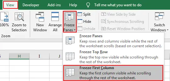
Freeze panes to lock rows and columns
To keep an area of a worksheet visible while you scroll to another area of the worksheet, go to the View tab, where you can Freeze Panes to lock specific rows and columns in place, or you can Split panes to create separate windows of the same worksheet.

Freeze rows or columns
Freeze the first column
-
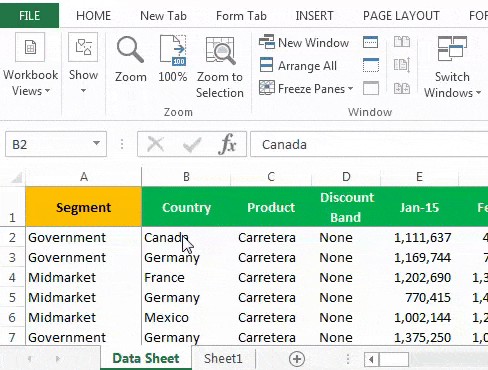
Select View > Freeze Panes > Freeze First Column.
The faint line that appears between Column A and B shows that the first column is frozen.
Freeze the first two columns
-
Select the third column.
-
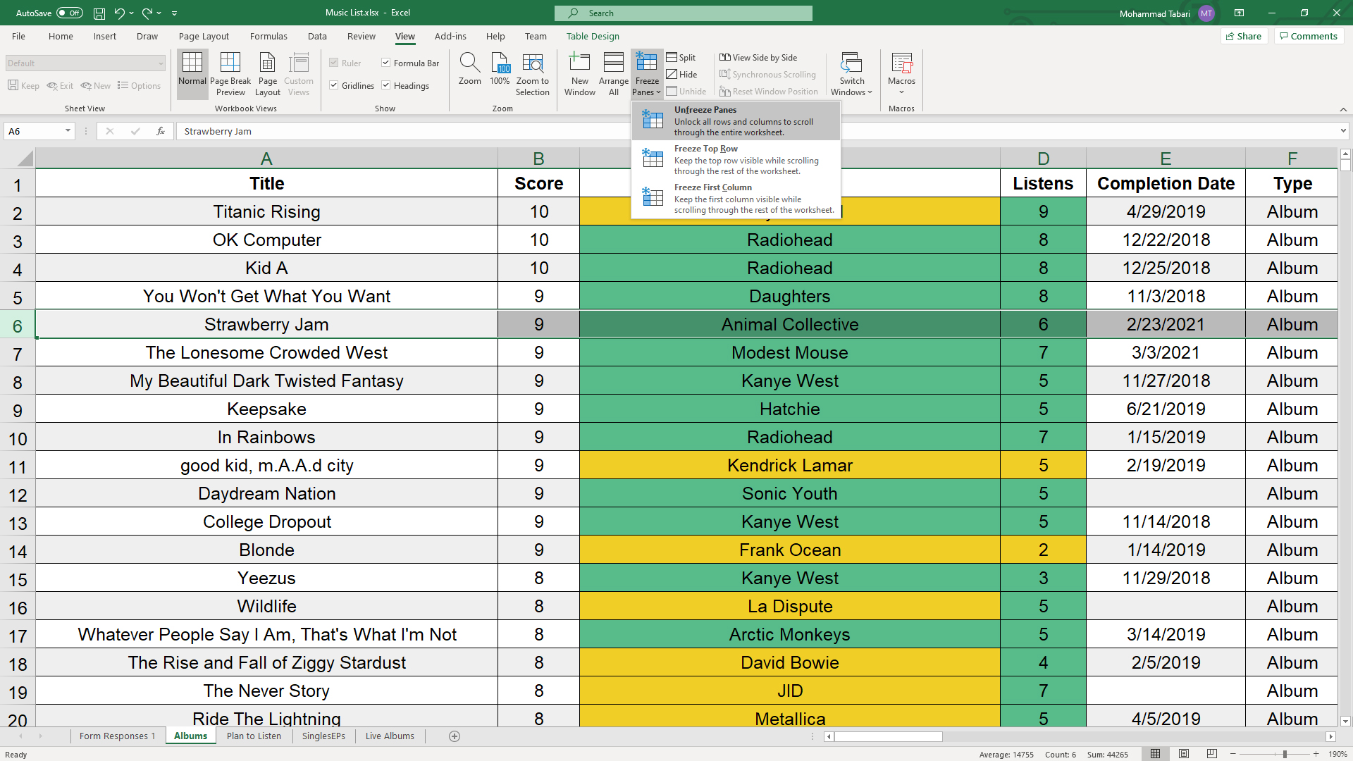
Select View > Freeze Panes > Freeze Panes.
Freeze columns and rows
-
Select the cell below the rows and to the right of the columns you want to keep visible when you scroll.
-
Select View > Freeze Panes > Freeze Panes.
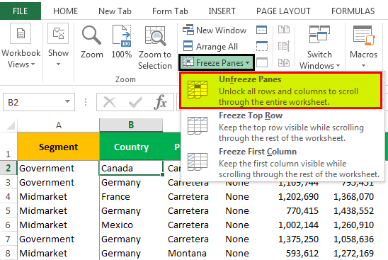
Unfreeze rows or columns
-
On the View tab > Window > Unfreeze Panes.

Note: If you don’t see the View tab, it’s likely that you are using Excel Starter. Not all features are supported in Excel Starter.

Need more help?
You can always ask an expert in the Excel Tech Community or get support in the Answers community.
See Also
Freeze panes to lock the first row or column in Excel 2016 for Mac
Split panes to lock rows or columns in separate worksheet areas
Overview of formulas in Excel
How to avoid broken formulas
Find and correct errors in formulas
Keyboard shortcuts in Excel
Excel functions (alphabetical)
Excel functions (by category)
Need more help?
Want more options?
Explore subscription benefits, browse training courses, learn how to secure your device, and more.
Communities help you ask and answer questions, give feedback, and hear from experts with rich knowledge.
Freezing columns in excel fixes or locks them so that they remain visible while scrolling through the database. A frozen column does not move with the movement of the remaining columns.
For example, freezing the first column (column A) ensures that it stays at its place at the time of navigation through the rest of the columns. Moreover, if column A consists of headings, the user may want to view these while working on the other columns of the dataset.
The objectives of freezing an excel column are:
- To ensure that the user does not lose track of the specific column
- To facilitate comparison of different columns of the worksheet
Freezing columns prevents the user from referring to the same column again and again. In other words, the frozen columns save the scrolling time of the user.
All the properties of the frozen column apply to the frozen row as well.
The “freeze panesFreezing panes in excel helps freeze one or more rows and/or columns so that they remain fixed while scrolling through the database.read more” drop-down under the View tab lists the following options:
- Freeze panes–It freezes multiple rows and columns.
- Freeze top row–It freezes only the first row.
- Freeze first column–It freezes only the first column.
After freezing a row or column in excel, a grey line appears at the end of the frozen area. This line indicates that the row or column has been frozen.
Table of contents
- #1 Freeze the First Column in Excel
- Example #1
- #2 Freeze Multiple Columns in Excel
- Example #2
- #3 Freeze the Row and Column Together in Excel
- Example #3
- #4 Unfreeze Panes in Excel
- The Rules of Freezing in Excel
- Frequently Asked Questions
- Recommended Articles
Let us go through the ways of freezing the first excel column, multiple columns, and both rows and columns.
#1 Freeze the First Column in Excel
Freezing the first column locks column A of the worksheet. This means that on moving from left to right, this column will be visible at all times.
In addition, column A is fixed irrespective of the column from which the actual data begins. The excel shortcut to freeze the first column is “Alt+W+F+C” (when pressed one by one).

Let us consider an example.
Example #1
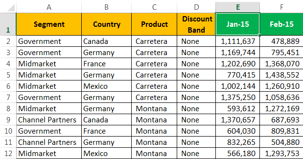
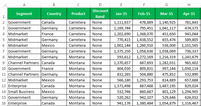
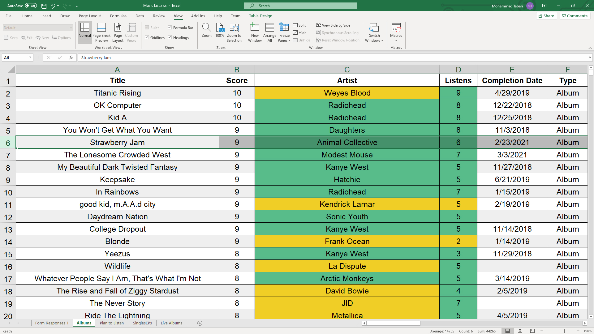
The following table shows the sales revenue (in $) generated by the products of specific segments. The data relates to various countries and is spread across the first five months of the year 2015.
We want to freeze the first excel column (column A).
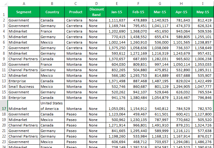
In order to view the column “segment” on a movement from left to right, we need to freeze it.
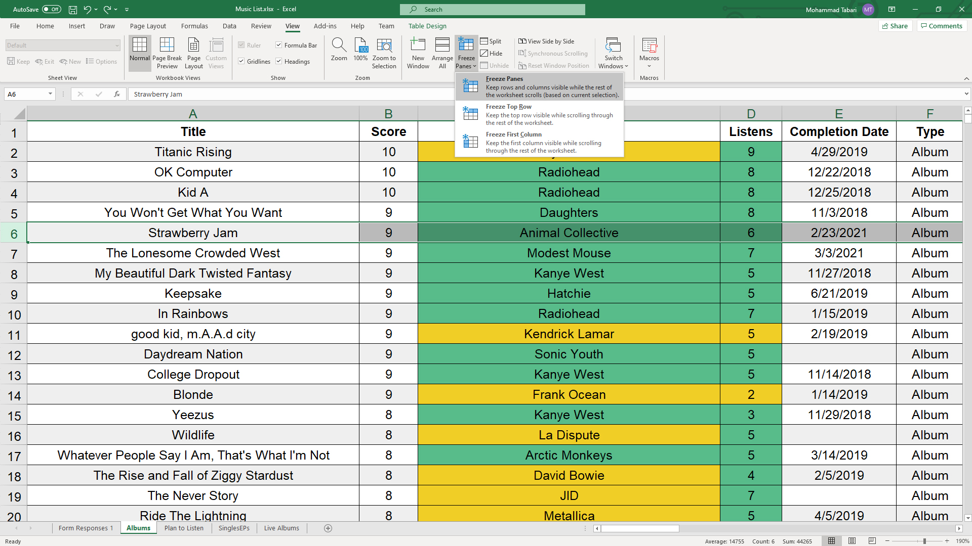
The steps for freezing the excel column are listed as follows:
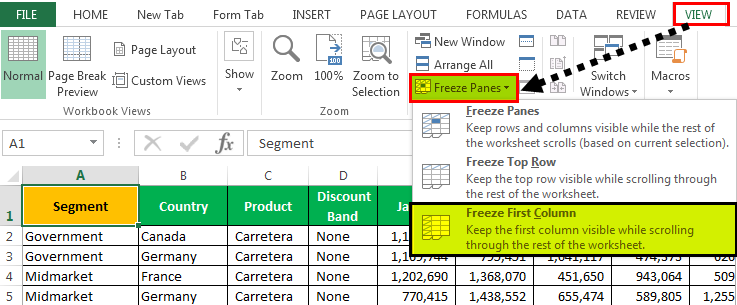
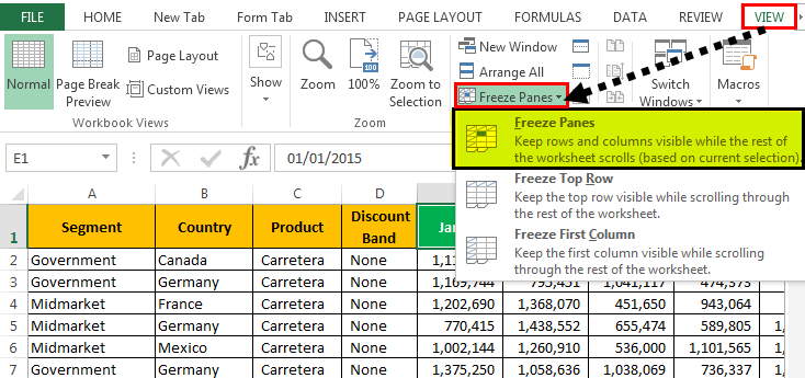
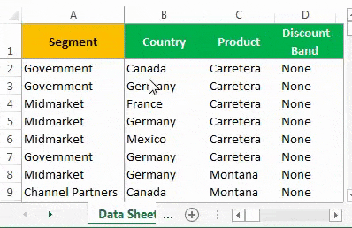
- Select the worksheet where the first column is to be frozen.
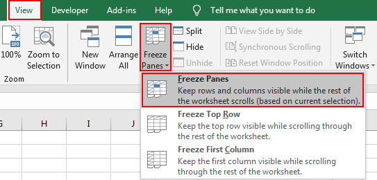
- In the View tab, click the “freeze panes” drop-down under the “window” section. Select “freeze first column,” as shown in the succeeding image.
Alternatively, press the shortcut keys “Alt+W+F+C” one by one.

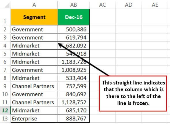
- The first column is frozen. The grey line appears at the end of column A indicating that the column to the left is frozen. The column AB shown in the following image is the last scrolled column of the dataset.

- On scrolling (from left to right) through the remaining columns of the dataset, column A is visible. The same is shown in the following image.

In the same way, the first row can be frozen.
#2 Freeze Multiple Columns in Excel
Freezing multiple excel columns is similar to freezing multiple rows. For freezing multiple columns, select the first right-hand side cell immediately after the last column to be frozen. This is because multiple columns are frozen based on the current selection.
Similarly, for freezing multiple rows, select the first cell immediately below the last row to be frozen.
For example, to freeze the columns A, B, and C, select the cell D1. By freezing the first three columns, they remain visible to the user at all times. Likewise, to freeze the rows 1, 2, and 3, select the cell A4.
The shortcut to freeze multiple excel columns is “Alt+W+F+F” (when pressed one by one).

Let us consider an example.
Example #2
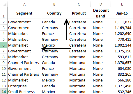
Working on the data of example #1, we want to freeze the first four columns, A, B, C, and D.
The steps for freezing multiple excel columns are listed as follows:
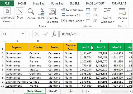
Step 1: Select the cell E1. This is because the first four columns are to be frozen.
Step 2: In the View tab, click the “freeze panes” drop-down under the “window” section. Select “freeze panes,” as shown in the succeeding image.
Alternatively, press the shortcut keys “Alt+W+F+F” one by one.
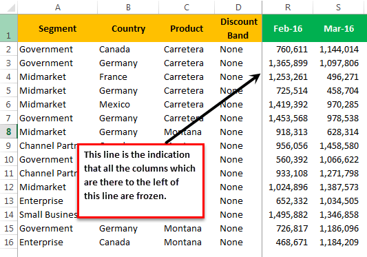
Step 3: The first four columns are frozen. The grey line appears (shown in the following image) at the end of column D, indicating that the columns to the left are frozen.
The columns R and S shown in the following image are the scrolled columns towards the end of the dataset.
Step 4: On scrolling (from left to right) till the last column of the dataset, the first four columns are visible. The same is shown in the following image.
#3 Freeze the Row and Column Together in Excel
Usually, the first row and the first column of a database contain headers. The user might want to view the row 1 and the column A simultaneously and at all times. Hence, it is essential to lock them together to permit their visibility while scrolling down and from left to right.
The only difference between the methods #2 and #3 is in the selection of the cell (step 1). With the “freeze panes” option, Excel freezes the rows and columns preceding the current active cell.
The shortcut to freeze the row and column together is “Alt+W+F+F” (when pressed one by one).
Let us consider an example.
Example #3
Working on the data of example #1, we want to freeze the first row (row 1) and the first column (column A) at the same time.
The steps to freeze the excel row 1 and column A together are listed as follows:
Step 1: Select the cell B2.
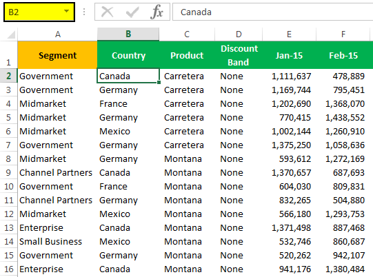
Step 2: Press the shortcut keys “Alt+W+F+F” one by one. It freezes the column to the left of the selected cell B2. At the same time, the row preceding the active cell (B2) is also frozen, as shown in the following image.
Hence two grey lines appear, one at the end of row 1 (horizontal) and the other at the end of column A (vertical).
Note: Alternatively, the “freeze panes” option can be selected from the “freeze panes” drop-down of the View tab.
Step 3: On scrolling from top to bottom and left to right, the row 1 and column A are visible. The same is shown in the following image.
Note: It is possible to freeze as many rows and columns depending on the requirement. The condition is that freezing of multiple excel rows and columns should begin with the top row (row 1) and the first column (column A).
#4 Unfreeze Panes in Excel
Unfreezing of panes does not require any cells to be selected. The steps to unfreeze panes in Excel are listed as follows:
Step 1: In the View tab, click the “freeze panes” drop-down under the “window” section. Select “unfreeze panes,” as shown in the succeeding image.
Alternatively, press the shortcut keys “Alt+W+F+F” one by one.
Step 2: The grey lines are removed, as shown in the following image.
Note: The “unfreeze panes” option appears only after freezes have been applied to the Excel worksheet.
The Rules of Freezing in Excel
The norms governing the freezing of rows and columns are listed as follows:
- It is not possible to freeze excel rows and columns in the middle of the worksheet.
- The option “freeze panes” can be applied only once. It is not possible to create multiple “freeze panes” in a single worksheet.
- The rows and columns to be fixed should be visible at the time of freezing. Otherwise, they will remain hidden even after freezing.
Note 1: To divide a worksheet into two or more areas with separate scroll barsIn Excel, there are two scroll bars: one is a vertical scroll bar that is used to view data from up and down, and the other is a horizontal scroll bar that is used to view data from left to right.read more for each, use the “split” option. This is available in the “window” section of the View tab.
Note 2: To fix the header row of a large dataset that does not fit into the screen, create an Excel tableIn excel, tables are a range with data in rows and columns, and they expand when new data is inserted in the range in any new row or column in the table. To use a table, click on the table and select the data range.read more. Moreover, ensure the visibility of this row by selecting any cell within the table before scrolling.
Frequently Asked Questions
1. What does freezing columns mean and how to freeze the first column in Excel?
Freezing a column means locking it in order to keep it visible while the user scrolls through the database. This is specifically helpful if a column contains headers which are required to be seen at all times.
After freezing, a grey line appears to indicate the frozen columns on its left. The steps to freeze the first column (column A) are listed as follows:
• In the View tab, click the “freeze panes” drop-down under the “window” section.
• Select “freeze first column.” Alternatively, press the shortcut keys “Alt+W+F+C” one by one.
• The first column (column A) is frozen.
Note: For freezing the first row, select “freeze top row” from the “freeze panes” drop-down of the View tab.
2. How to freeze multiple columns in Excel?
Let us freeze columns A, B, C, D, and E. The steps to freeze multiple columns in Excel are listed as follows:
• Select either the column or the first cell to the right of the last column to be frozen (column E). So, select either column F or the cell F1.
• In the View tab, click the “freeze panes” drop-down under the “window” section.
• Select “freeze panes.” Alternatively, press the shortcut keys “Alt+W+F+F” one by one.
• The columns A B, C, D, and E are frozen as indicated by the grey line at the end of column E.
3. How to freeze rows and columns together in Excel?
Let us freeze rows 1, 2, and 3 and columns A, B, and C. The steps to freeze the given rows and columns together are listed as follows:
• Select cell D4 based on the following parameters:
a. It immediately follows the last row to be frozen (row 3).
b. It is to the right of the last column to be frozen (column C).
• In the View tab, click the “freeze panes” drop-down under the “window” section.
• Select “freeze panes.” Alternatively, press the shortcut keys “Alt+W+F+F” one by one.
• The rows 1, 2, and 3 and columns A, B, and C are frozen. This is indicated by the grey line appearing below row 3 and at the end of column C.
Note: The freezing of multiple excel rows and columns should begin with the top row (row 1) and the first column (column A).
Recommended Articles
This has been a guide to freezing columns in Excel. Here we discuss how to freeze the first column, multiple columns, and both rows and columns. For more on Excel, take a look at the following articles-
- Adding Columns in ExcelAdding a column in excel means inserting a new column to the existing dataset.read more
- Group Excel ColumnsIn Excel, grouping one or more columns together in a worksheet is referred to as group column and I t allows you to contract or expand the column.read more
- Column Lock in ExcelThe Column Lock feature in Excel is designed to prevent any mishaps or unwanted modifications in data caused by a user’s mistake. It may be used on single or multiple columns, with cell formatting ranging from locked to unlocked, and the workbook can be password protected.read more
- Column Sort in Excel
When you’re working with a lot of spreadsheet data on your laptop, keeping track of everything can be difficult. It’s one thing to compare one or two rows of information when dealing with a small subset of data, but when a dozen rows are involved, things get unwieldy. And we haven’t even started talking about columns yet. When your spreadsheets become unmanageable, there’s only one solution: freeze the rows and columns.
Freezing rows and columns in Excel makes navigating your spreadsheet much easier. When done correctly, the chosen panes are locked in place; this means those specific rows are always visible, no matter how far you scroll down. More often than not, you’ll only freeze a couple of rows or a column, but Excel doesn’t limit how many of either you can freeze, which can come in handy for larger sheets.
This how-to works with Microsoft Excel 2016 as well as later versions. However, the this method also works with Google Sheets, OpenOffice and LibreOffice. Ready to get to work? Here’s how to freeze rows and columns in Excel:
- More: How to put Windows 10 into Safe Mode
- Here’s how to lock cells in Excel and how to recover a deleted or unsaved file in Excel
- This is how to use VLOOKUP in Excel and add additional rows above or below in Excel
How to freeze a row in Excel
1. Select the row right below the row or rows you want to freeze. If you want to freeze columns, select the cell immediately to the right of the column you want to freeze. In this example, we want to freeze rows 1 to 5, so we’ve selected row 6.
2. Go to the View tab. This is located at the very top, inbetween «Review» and «Add-ins.»
3. Select the Freeze Panes option and click «Freeze Panes.» This selection can be found in the same place where «New Window» and «Arrange All» are located.
That’s all there is to it. As you can see in our example, the frozen rows will stay visible when you scroll down. You can tell where the rows were frozen by the green line dividing the frozen rows and the rows below them.
If you want to unfreeze the rows, go back to the Freeze Panes command and choose «Unfreeze Panes».
Note that under the Freeze Panes command, you can also choose «Freeze Top Row,» which will freeze the top row that’s visible (and any others above it) or «Freeze First Column,» which will keep the leftmost column visible when you scroll horizontally.
Besides allowing you to compare different rows in a long spreadsheet, the freeze panes feature lets you keep important information, such as table headings, always in view.
Need more Excel tricks? Check out our tutorials on How to Lock Cells in Excel and How to Use VLOOKUP in Excel.
Get instant access to breaking news, the hottest reviews, great deals and helpful tips.
I recently helped a friend with Excel, and when I asked him how the spreadsheet looked, he hesitated. Finally, he looked at me and said, “It’s overwhelming.” The data was OK, but he wanted to see the top row when he scrolled. The solution was to show him how to freeze rows and columns in Excel so that key headings or cells were always visible. I’ve outlined four scenarios and solution steps.
This was a good communication lesson for me. It reminded me that we all have different skill levels and vocabularies. For example, when you’re new, you’re probably not thinking in terms like “how to freeze panes in Excel.” You may not know what a pane is. It’s not describing your problem. My friend was thinking in terms of a “sticky header,” or “Excel floating header,” or “pinning rows.” I wasn’t thinking of any of those.
Let’s Start with Excel Panes
An Excel pane is a set of columns and rows defined by cells. You get to determine the size, shape, and location. For many people, it might be the top row. For others, it’s an inverted L-shape and contains the top row and first column. You’re the spreadsheet architect and can define your pane.
Regarding spreadsheets, you can “freeze panes” or “split panes.” Splitting panes is a bit more complex because you have separate windows of your data on the worksheet. So, for the sake of simplicity, this tutorial will cover freezing panes.
If your columns and rows aren’t in the orientation you want, you may want to learn how to transpose or switch columns and rows in Excel.
Why Lock Spreadsheet Cells?
A key benefit to locking or freezing cells is seeing the important information regardless of scrolling. The split pane data stays fixed. Your spreadsheet can contain panes with column headings, multiple rows, multiple columns, or both.
Otherwise, losing focus on a large worksheet is easy when you don’t have column headings or identifiers. I’ve had times where I’ve entered data only to see I was one cell off and produced Excel formula errors. By locking various sections, you have a consistent reference point. This also helps readability.
Typically, the cells you want to stay sticky are labels like headers. However, they could just as easily be an entire column, such as employee names.
Let’s go through four examples and keyboard shortcuts to freeze panes in Excel.
1 – How to Freeze the Top Row
This freeze row example is perhaps the most common because people like to lock the top row that contains headers, such as in the example below.
Another solution is to format the spreadsheet as an Excel table.
- Open your worksheet.
- Click the View tab on the ribbon.
- On the Freeze Panes button, click the small triangle ▼ (drop-down arrow) in the lower right corner. You should see a new menu with three options.

- Click the menu option Freeze Top Row.
- Scroll down your sheet to ensure the first row stays locked at the top.
You should see a darker border under row 1.
Keyboard Shortcut – Lock Top Row
I like to do this shortcut slowly the first time to see the ALT key letter assignments as you type. I can see the keyboard assignments in the example below once I hit my Alt key. Some people prefer to add the Freeze Panes command to the Quick Access toolbar because they frequently use it.

Alt + w + f + r
2 – How to Freeze the First Column
A similar scenario is when you want to freeze the leftmost column. I guess Microsoft researched this to determine the most common sub-menu options.
I find this option helpful when I have a spreadsheet with many columns and I need to fill in data without using an Excel data form.

- Open your Excel worksheet.
- Click the View tab on the ribbon.
- On the Freeze Panes button, click the small triangle ▼. You should see a new menu with your 3 options.
- Click the option Freeze First Column.
- Scroll across your sheet to make sure the left column stays fixed.
Keyboard Shortcut – Lock First Column
Alt + w + f + c
3 – How to Freeze the Top Row & First Column
This is my favorite option. If you look at Microsoft’s initial Freeze Panes options, there isn’t one for the top row and first column. Instead, we’ll use the generic option called Freeze Panes.
The subtext reads, “Keep rows and columns visible while the rest of the worksheet scrolls (based on current selection).” Some folks get confused as they think they have to highlight data to make a selection.
Instead, consider the selection of the first cell outside your fixed column and row. If I wanted to lock the top row and top column, that selection cell would be cell B2 or Nevada. Regardless of whether I scroll down or to the right, the first cell that disappears when I scroll is B2.

- Open your Excel spreadsheet.
- Click cell B2. (Your set cell.)
- Click the View tab on the ribbon.
- On the Freeze Panes button, click the small triangle ▼ in the lower right corner. You should see a dropdown menu with your 3 options.
- Click the option Freeze Panes.
- Scroll down your worksheet to make sure the first row stays at the top.
- Scroll across your sheet to make sure your first column stays locked on the left.
Keyboard Shortcut – Freeze Panes
Alt + w + f + f
4 – Freeze Multiple Columns or Rows
On occasion, I get some Excel worksheets where the author puts descriptive text above the data. My header isn’t in Row 1 but further down in Row 5. Or I want to lock multiple columns to the left. In the example below, I want to lock Columns A & B and Rows 1-5.

The process is the same, I just need to click the set cell that stops the fixed area. In this case, it would be cell C6 or “Regions Field.” The content above and to the left is frozen.
Everything in the red boxes would be locked. The downside is you may give up much of the screen real estate.
Why Freeze Panes May Not Work
There are some rules surrounding this feature. If you don’t follow these, freeze panes may not work.
Quick test: If you type Ctrl + Home and your cursor moves to cell A1, you haven’t locked anything.
- If you dislike your settings, use the Unfreeze Panes command.
- This feature won’t work on a protected worksheet or Page Layout View.
- If you’re editing a value in the Formula bar, the View menu will be disabled.
If you need to see the same header on printed pages, Microsoft has instructions.
As you’ve seen, choosing what content to freeze is easy. You can freeze the top row, first column, both, or a subset of your data, depending on what you want to do with it. The flexibility is part of what makes Microsoft Excel such an excellent program for organizing and analyzing information from any field.
![]()
Download Article
![]()
Download Article
- Freezing the First Column or Row
- Freezing Multiple Columns or Rows
- Video
- Q&A
|
|
|
This wikiHow teaches you how to freeze specific rows and columns in your Microsoft Excel worksheet. Freezing rows or columns ensures that certain cells remain visible as you scroll through the data. If you want to easily edit two parts of the spreadsheet at once, splitting your panes will make the task much easier.
-
1
Click the View tab. It’s at the top of Excel. Frozen cells are rows or columns that remain visible while you scroll through a worksheet.[1]
If you want column headers or row labels to remain visible as you work with large amounts of data, you’ll likely find it helpful to lock those cells into place.- Only whole rows or columns can be frozen. It is not possible to freeze individual cells.
-
2
Click the Freeze Panes button. It’s in the «Window» section of the toolbar. A set of three freezing options will appear.
Advertisement
-
3
Click Freeze Top Row or Freeze First Column. If you want to keep the top row of cells in place as you scroll down through your data, select Freeze Top Row. To keep the first column in place as you scroll horizontally, select Freeze First Column.
-
4
Unfreeze your cells. If you want to unlock the frozen cells, click the Freeze Panes menu again and select Unfreeze Panes.


Advertisement
-
1
Select the row or column after those you want to freeze. If the data you want to keep stationary takes up more than one row or column, click the column letter or row number after those you want to freeze. For example:
- If you want to keep rows 1, 2, and 3 in place as you scroll down through your data, click row 4 to select it.
- If you want columns A and B to remain still as you scroll sideways through your data, click column C to select it.
- Frozen cells must connect to the top or left edge of the spreadsheet. It’s not possible to freeze rows or columns in the middle of the sheet.[2]
-
2
Click the View tab. It’s at the top of Excel.
-
3
Click the Freeze Panes button. It’s in the «Window» section of the toolbar. A set of three freezing options will appear.
-
4
Click Freeze Panes on the menu. It’s at the top of the menu. This freezes the columns or rows before the one you selected.
-
5
Unfreeze your cells. If you want to unlock the frozen cells, click the Freeze Panes menu again and select Unfreeze Panes.


Advertisement
Add New Question
-
Question
How do I freeze the top two rows?

Select the row directly under the rows you want to freeze (in this case, the third row). Go to View, Freeze Panes, and select «Freeze Panes.» Everything above the row you have selected will be frozen.
Ask a Question
200 characters left
Include your email address to get a message when this question is answered.
Submit
Advertisement
Thanks for submitting a tip for review!
wikiHow Video: How to Freeze Cells in Excel
About This Article
Article SummaryX
1. Click View.
2. Click Freeze Panes.
3. Select Freeze Top Row or Freeze First Column.
Did this summary help you?
Thanks to all authors for creating a page that has been read 171,421 times.
Is this article up to date?
Just assume you are school teacher and have around 90 students in a class which is divided into various sections. Now, you have to collate their marks in every subject in an excel.
If you are using a 15-inch laptop to do this, then as soon as you go to the 25th row or later you lose the context of which column is for which subject. All of this happens because your header or first row is not fixed and keeps changing as you scroll down. But don’t worry we are here to help you out. 🙂
In this post we are going to help you on how to freeze rows or columns in excel. Freeing in excel will turn some cells (rows and / or columns) to be stagnant and these cells would not change if you move left or right or scroll up or down. There are various ways to freeze cells in excel.

We have listed all the methods below, if you do not want to go through the entire post then you may directly click on the type of excel freeze option you are looking for:
- Freeze First Row
- Freeze First Column
- Freeze Panes
- Freeze Multiple Rows
- Freeze Multiple Columns
- Freeze Rows & Columns at same time
Along with helping you on how to freeze in excel, we will also help you to unfreeze and troubleshooting issues that you might encounter:
- Unfreeze Panes
- Freeze panes versus Splitting Panes
- Freeze Pane is Disabled
Freeze First Row
This feature could be used to freeze a particular row or header that you would need to refer every time while working on excel. In this option only the top row will freeze.
- Open the sheet where in you want to freeze any row / header, as an example we would like to freeze the top row highlighted in yellow

- Now, navigate to the “View” tab in the Excel Ribbon as shown in above image
- Click on the “Freeze Panes” button

- Select “Freeze Top Row” option

- If you would like to freeze any other row, then scroll down and make that row appear as first in your sheet and then repeat Step 2 to 4.
That’s it. You are all set now. As seen in above image you can now scroll to any corner of the page and you would see that the top row remains intact all the time without any change.
Please note that this option works as long as first row in excel is the one that you really want to freeze. If you have scrolled in the middle of the sheet and Row 30 is appearing as first row, then this option would freeze Row 30 and not Row 1.
Additionally, if you are geek and would like to do it directly using a keyboard shortcut, then please press “Alt + W” followed by “F” and then “R”. Please note that this is not an in-built shortcut, rather it’s the same thing from keyboard as we do from mouse.
Freeze First Column
This feature could be used to freeze a particular column that you would need to refer while working on excel. In this option only the first column will freeze.
- Open the sheet where in you want to freeze the column, as an example we would like to freeze the column A – Product

- Now, navigate to the “View” tab in the Excel Ribbon as shown in above image
- Click on the “Freeze Panes” button

- Select “Freeze First Column” option

- If you would like to freeze any other column, then move right or left and make that column appear as first in your sheet and then repeat Step 2 to 4.
That’s it. You are all set now. As seen in above image you can now move to most right corner of the page and you would see that the first column sticks there. Please note that this option works as long as first column in excel is the one that you really want to freeze. If you have shifted right in the middle of the sheet and Column M is appearing as first row, then this option would freeze Column M and not Column A.
If you would like to do it directly using a keyboard shortcut, then please press “Alt + W” followed by “F” and then “C”. Please note that this is not an in-built shortcut, rather it’s the same thing from keyboard as we do from mouse.
Freeze Panes
This feature could be used to freeze multiple rows, columns or both at the same time. However, this could be done only for the consecutive rows or columns.
Freeze Panes – Multiple Rows
- Open the sheet where in you want to freeze the multiple rows, keep the first row on top and click after the last row till where you want to freeze, as an example we would like to freeze from Row 1 to Row 13 so we will click on Row 14

- Now, navigate to the “View” tab in the Excel Ribbon as shown in above image
- Click on the “Freeze Panes” button

- Select “Freeze Panes” option

That’s it. You are all set now. As seen in above image you can now scroll down and Row 1 to Row 13 will be kept intact without any changes. You can select the range of rows from middle as well like – Row 13 to Row 30, however to do so you will have to ensure that you scroll up and keep Row 13 as your first row in the sheet and repeat the steps listed above. However, be careful as doing so some of your rows (i.e. the ones before Row 13) will be hidden.
Freeze Panes – Multiple Columns
- Open the sheet where in you want to freeze the multiple columns, keep the first column to the left and click next to the last column till where you want to freeze, as an example we would like to freeze from Column A to E, so we will click on Column F

- Now, navigate to the “View” tab in the Excel Ribbon as shown in above image
- Click on the “Freeze Panes” button

- Select “Freeze Panes” option

That’s it. You are all set now. As seen in above image you can now move towards right and Column A to E will be kept intact without any changes. You can select the range of columns from middle as well like – Column F to Column L, however to do so you will have to ensure that you move to the left and keep Column F as your first column in the sheet and repeat the steps listed above. However, be careful as doing so some of your columns (i.e. the ones before Column E) will be hidden.
Freeze Panes – Multiple Rows and Columns both
If you have followed the post till now, then you would have already figured out how this has to be done. Yes, you are right we are going to club both the above listed approaches here. Follow us below:
- Open the sheet where in you want to freeze the multiple rows and columns, keep the first row on top and first column to the left then click next to the cell of the last column and row till where you want to freeze, as an example we would like to freeze from Row 1 to 13 and Column A to E, so we will click on Cell F14

- Now, navigate to the “View” tab in the Excel Ribbon as shown in above image
- Click on the “Freeze Panes” button

- Select “Freeze Panes” option

That’s it. You are all set now. As seen in above image you can now scroll down and Row 1 to 13 will remain intact and likewise you can move towards right and Column A to E will be kept intact without any changes. You can select the range of columns from middle as well like – Row 17 to 27 and Column F to L, however to do so you will have to ensure that you scroll up and keep Row 17 as your first row and keep Column F as your first column in the sheet and repeat the steps listed above. Be careful here as rows before Row 17 and columns before column F will be hidden.
Unfreeze Panes:
If you have frozen the wrong rows and columns, then you could easily undo it by using “Unfreeze Panes” option. This would remove all the frozen rows and or columns in your excel. This will also work if you have received the sheet from someone else and you are not able to see all the rows and columns despite of removing all filters and unhiding rows columns. To unfreeze panes –
- Open the sheet wherein you want to unfreeze rows and or columns
- Now, navigate to the “View” tab in the Excel Ribbon
- Click on the “Freeze Panes” button

- Select “Unfreeze Panes” option as shown above

With this all the rows and or columns would unfreeze, as shown in above image. Please note that you would not see the “Unfreeze Panes” option if there are not any frozen rows columns. This option would be available only and only when there is some row and or column frozen already.
If you would like to unfreeze panes it directly using a keyboard shortcut, then please press “Alt + W” followed by “F” and then again “F”. Please note that this is not an in-built shortcut, rather it’s the same thing from keyboard as we do from mouse.
Freeze panes versus Splitting Panes:
Excel also provides you an excellent option to Split Panes which divides the window into different panes that each pane scrolls separately. This option is present in Excel Ribbon, View tab next to Freeze Option.

So as visible in the above image after using split option the content of same sheet is visible in 4 separate panes and all panes have their different scroll options.
We personally trust and use Freeze option much than Split, as Freeze allows you to limit the data movement by freezing it rather than adding multiple views of same data wherein you easily get distracted and confused while data entry.
Is Freeze Pane option disabled?
If you have come across a case wherein the Freeze Pane option is disabled in your sheet, then it must be due to one of the following reasons:
- The most common reason of Freeze Panes option disablement is that your sheet must have been opened in “Page Layout” mode (as shown in below image)

In order to correct it simply navigate to “View Tab” in the excel ribbon and select “Normal” or “Page Break” view.
- The “Freeze Panes” option could also be disabled if you excel has been protected for windows. You would need to unprotect it to enable the freeze option.
So, this was all about how to freeze rows and columns in Excel. Hope you enjoyed our tutorial. Please feel free to share your feedback and queries. Keep Exceling 🙂
Watch Video – Using Excel Freeze Panes
When working with large data sets, if you scroll down or to the right of the worksheet you would lose track of the row/column headings.
In such situations, you can use the Excel Freeze Panes feature to freeze the rows or columns in your dataset – so that the headers always visible no matter where you scroll in your data.
Accessing Excel Freeze Panes Options
To access Excel Freeze Panes options:
It shows three options in the Freeze Panes drop-down:
- Freeze Panes: It freezes the rows as well as the columns.
- Freeze Top Row: It freezes all the rows above the active cell.
- Freeze First Column: It freezes all the columns to the left of the active cell.
You can use these options to lock rows or columns (or both) into panes in Excel.
Let’s see how to use these options to Freeze Panes in Excel while working with large data sets:
Freezing Row(s) in Excel
If you are working with a dataset that has headers at the top row and a dataset that spans hundreds of rows, as soon as you scroll down, the headers/labels would disappear.
Something as shown below:
In such cases, it’s a good idea to freeze the header row so that these are always visible to the user.
In this section, you’ll learn how to:
- How to Freeze the top row.
- How to Freeze more than one row.
- How to Unfreeze rows.
Freeze the Top Row in Excel
Here are the steps to freeze the first row in your dataset:
Now when you scroll down, the row that has been frozen would always be visible. Something as shown below:

Freeze/Lock More than One Row in Excel
If you have more than one header rows in your dataset, you may want to freeze all of it.
Here is how to freeze rows in Excel:
- Select the left-most cell in the row which is just below the headers row.
- Click the ‘View’ tab.
- In the Zoom category, click on the Freeze panes drop down

- In the Freeze Panes drop-down, select Freeze Panes.

- This will freeze all the rows above the selected cell. You would notice that a gray line now appears right below the rows that have been freezed.

Now when you scroll down, all the header rows would always be visible. Something as shown below:

Also read: How to Freeze Multiple Columns in Excel?
Unfreeze Rows in Excel
To unfreeze row(s):
Excel Freeze Panes Options – Freezing Column(s)
If you are working with a dataset that has headers/labels in a column and the data is spread across many columns, as soon as you scroll to the right, the header would disappear.
Something as shown below:

In such cases, it’s a good idea to freeze the left-most column so that the headers are always visible to the user.
In this section, you’ll learn how to:
- How to Freeze the Left-most Column.
- How to Freeze more than one Column.
- How to Unfreeze Columns.
Freeze/Lock the Left-Most Column in Excel
Here is how to freeze the left-most column:
Now when you scroll down, the left-most column would always be visible. Something as shown below:

Additional Notes:
- Once you freeze a column, you can not use Control + Z to unfreeze it. You need to use the unfreeze option in the Freeze Panes drop-down.
- If you insert a column to the left of the column that has been frozen, even the inserted column is frozen.
Freeze/Lock More than One Column in Excel
If you have more than one column that contains headers/labels, you may want to freeze all of it.
Here is how to do this:
- Select the top-most cell in the column which is right next to the columns that contain headers.
- Click the ‘View’ tab.
- In the Zoom category, click on the Freeze panes drop-down
- In the Freeze Panes drop-down, select Freeze First Column.

- This will freeze all the columns to the left of the selected cell. You would notice that a gray line appears to the right of the columns that have been frozen.
Now when you scroll to the right, all the columns with headers would always be visible. Something as shown below:

Unfreeze Columns in Excel
To unfreeze column(s):
Freezing Both Row(s) & Column(s)
In most of the cases, you would have the headers/labels in rows as well as in columns. In such cases, it makes sense to freeze both rows and columns.
Here is how you can do this:
Now when you scroll down or to the right, the frozen rows and columns would always be visible. Something as shown below:

You can unfreeze the frozen rows and columns at one go. Here are the steps:
Notes:
- Apart from working with large data sets, one practical use where you may want to freeze panes in Excel is when you are creating dashboards. You can freeze rows and columns that contain the dashboard so that the user can’t scroll away and the dashboard is always visible.
- A good practice while working with large data sets is to convert it into Excel Tables. By default, all the row headers in Excel Tables are always visible when you scroll within the dataset.
You May Also Like the Following Excel Tutorials:
- Excel Data Entry Tips
- How to Lock Cells in Excel.
- How to Lock Formulas in Excel.
- Compare Columns in Excel
- Move Rows and Columns in Excel
- Delete Blank Rows in Excel
- Highlight Rows Based on a Cell Value in Excel
- How to Turn OFF Scroll Lock in Excel?
Suppose we create a large table in excel spreadsheet and it lists large amount of data. There are headers in the first row, and if we want to drag the scroll bar to view the bottom of table, the headers are hidden due to it lists on the top. So, in this case if we want to see the headers all the time, we need to freeze the first row to make it fixed and always displays on the top even we drag the scrollbar. On the other side, sometimes we need to freeze more rows, or columns, or even freeze row and column simultaneously. To implement this, we need to know the way to freeze row and columns. This article will introduce different ways to freeze row and columns with examples for you, you can’t miss it.
Table of Contents
- Method 1: How to Freeze the First Row in Excel Spreadsheet
- Method 2: How to Freeze Multiple Rows in Excel Spreadsheet
- Method 3: How to Freeze the First Column in Excel Spreadsheet
- Method 4: How to Freeze Row and Column in Excel Spreadsheet
- Method 5: How to Freeze Rows and Columns in Excel Spreadsheet
Method 1: How to Freeze the First Row in Excel Spreadsheet
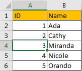
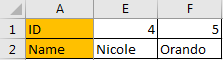
In most daily work, freeze the first row in table is frequently needed due to in most tables the first row lists the headers. So, people always want to see the headers on top no matter whether they drag the scrollbar to the end or not. See example below:
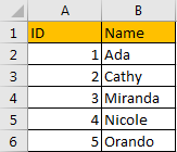
Suppose it lists a long list of ID and names. Header ID and Name are listed on the top. Now let’s freeze the first row.
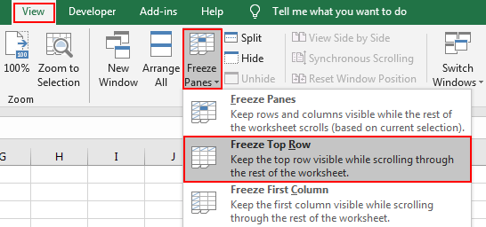
Step 1: Click View in the ribbon, then click Freeze Panes in Window group, then click the small triangle of Freeze Panes to load below three options, select the middle one ‘Freeze Top Row’.
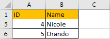
Step 2: After above operating. The first top row is fixed and always displayed on the top. Try to drag the scrollbar. You can see the header row is stayed on the top.
Method 2: How to Freeze Multiple Rows in Excel Spreadsheet
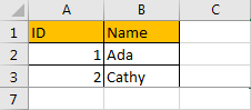
If you want to freeze the first three rows in excel, you can just select the first cell in the fourth row, then freeze the rows above the selected cell. See details below.
Step 1: Click A4 in the table.
Step 2: Click View in the ribbon, then click Freeze Panes in Window group, then click the small triangle of Freeze Panes to load below three options, select the first one ‘Freeze Panes’.
Step 3: Try to drag the scrollbar. Verify that top three rows are fixed.
Method 3: How to Freeze the First Column in Excel Spreadsheet
See screenshot below:
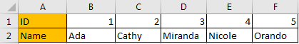
Now let’s freeze the first column. The way is similar with freeze the first row.
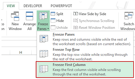
Step 1: Click View in the ribbon, then click Freeze Panes in Window group, then click the small triangle of Freeze Panes to load below three options, select the middle one ‘Freeze First Column’.
Step 2: Verify if it works well.
Obviously, it works.
Method 4: How to Freeze Row and Column in Excel Spreadsheet
If you want to just freeze the first row and column, just click on B2. Then click View->Freeze Panes->Freeze Panes in Window group.

Method 5: How to Freeze Rows and Columns in Excel Spreadsheet
If you want to freeze multiple rows and columns, refer to the description of Freeze Panes ‘Keep rows and column visible while the rest of the worksheet scrolls (based on current selection)’ we can know that we can select a cell to make it as the first cell outside of your fixed area. For example, if we want to freeze the top three rows and first two columns (row 4 is not fixed and column C is not fixed), we can click on C4, then repeat above steps to freeze panes.