
Freeze panes to lock rows and columns
To keep an area of a worksheet visible while you scroll to another area of the worksheet, go to the View tab, where you can Freeze Panes to lock specific rows and columns in place, or you can Split panes to create separate windows of the same worksheet.

Freeze rows or columns
Freeze the first column
-
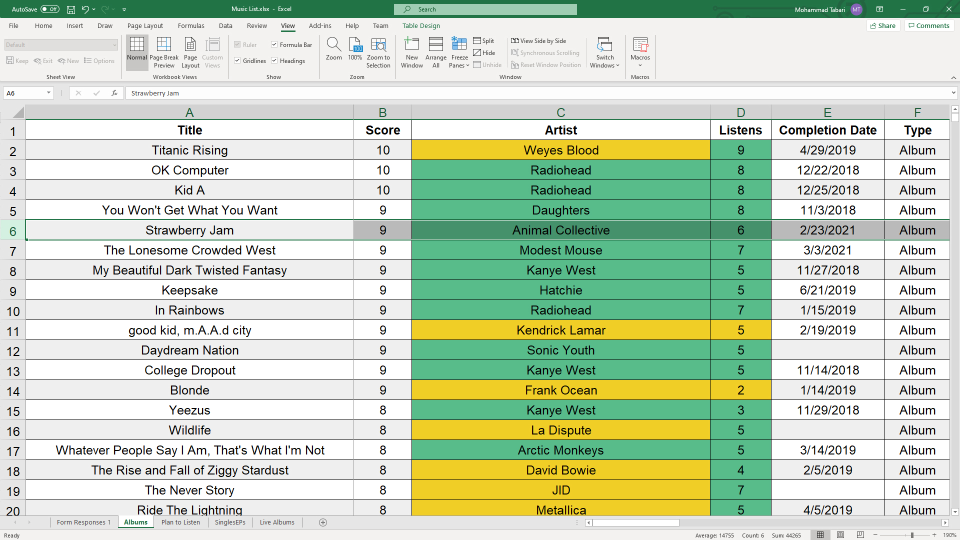
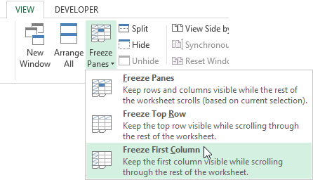
Select View > Freeze Panes > Freeze First Column.
The faint line that appears between Column A and B shows that the first column is frozen.
Freeze the first two columns
-
Select the third column.
-
Select View > Freeze Panes > Freeze Panes.
Freeze columns and rows
-
Select the cell below the rows and to the right of the columns you want to keep visible when you scroll.
-
Select View > Freeze Panes > Freeze Panes.
Unfreeze rows or columns
-
On the View tab > Window > Unfreeze Panes.

Note: If you don’t see the View tab, it’s likely that you are using Excel Starter. Not all features are supported in Excel Starter.

Need more help?
You can always ask an expert in the Excel Tech Community or get support in the Answers community.
See Also
Freeze panes to lock the first row or column in Excel 2016 for Mac
Split panes to lock rows or columns in separate worksheet areas
Overview of formulas in Excel
How to avoid broken formulas
Find and correct errors in formulas
Keyboard shortcuts in Excel
Excel functions (alphabetical)
Excel functions (by category)
Need more help?
Freezing columns in excel fixes or locks them so that they remain visible while scrolling through the database. A frozen column does not move with the movement of the remaining columns.
For example, freezing the first column (column A) ensures that it stays at its place at the time of navigation through the rest of the columns. Moreover, if column A consists of headings, the user may want to view these while working on the other columns of the dataset.
The objectives of freezing an excel column are:
- To ensure that the user does not lose track of the specific column
- To facilitate comparison of different columns of the worksheet
Freezing columns prevents the user from referring to the same column again and again. In other words, the frozen columns save the scrolling time of the user.
All the properties of the frozen column apply to the frozen row as well.
The “freeze panesFreezing panes in excel helps freeze one or more rows and/or columns so that they remain fixed while scrolling through the database.read more” drop-down under the View tab lists the following options:
- Freeze panes–It freezes multiple rows and columns.
- Freeze top row–It freezes only the first row.
- Freeze first column–It freezes only the first column.
After freezing a row or column in excel, a grey line appears at the end of the frozen area. This line indicates that the row or column has been frozen.
Table of contents
- #1 Freeze the First Column in Excel
- Example #1
- #2 Freeze Multiple Columns in Excel
- Example #2
- #3 Freeze the Row and Column Together in Excel
- Example #3
- #4 Unfreeze Panes in Excel
- The Rules of Freezing in Excel
- Frequently Asked Questions
- Recommended Articles
Let us go through the ways of freezing the first excel column, multiple columns, and both rows and columns.
#1 Freeze the First Column in Excel
Freezing the first column locks column A of the worksheet. This means that on moving from left to right, this column will be visible at all times.
In addition, column A is fixed irrespective of the column from which the actual data begins. The excel shortcut to freeze the first column is “Alt+W+F+C” (when pressed one by one).

Let us consider an example.
Example #1
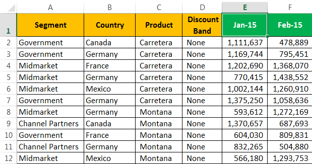
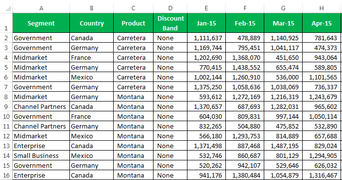
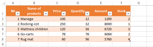
The following table shows the sales revenue (in $) generated by the products of specific segments. The data relates to various countries and is spread across the first five months of the year 2015.
We want to freeze the first excel column (column A).
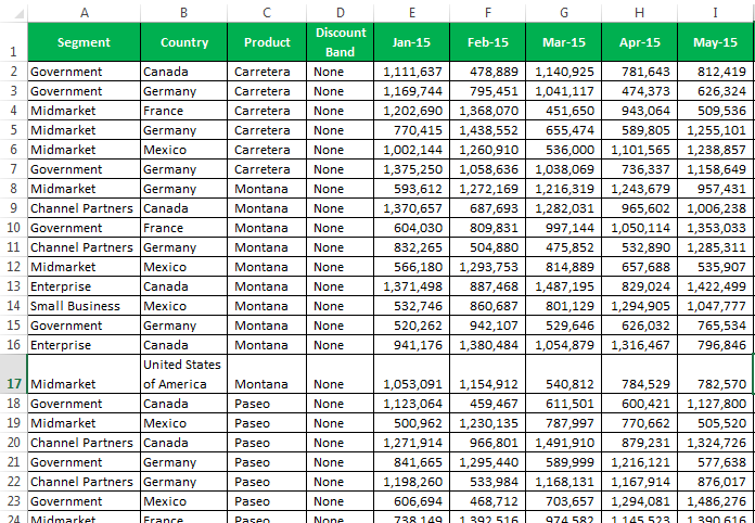
In order to view the column “segment” on a movement from left to right, we need to freeze it.
The steps for freezing the excel column are listed as follows:
- Select the worksheet where the first column is to be frozen.
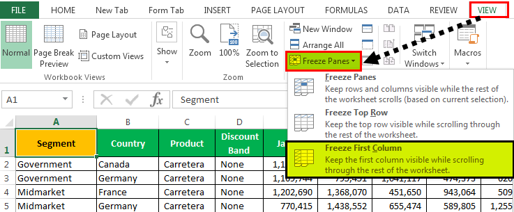
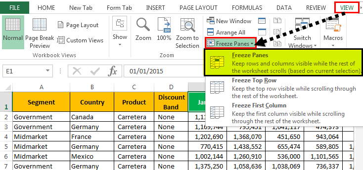
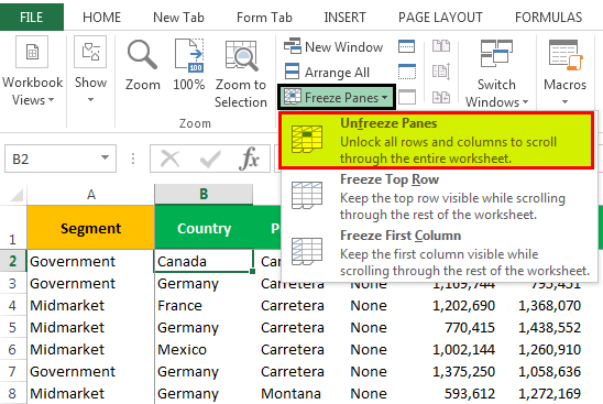
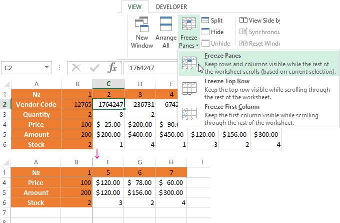
- In the View tab, click the “freeze panes” drop-down under the “window” section. Select “freeze first column,” as shown in the succeeding image.
Alternatively, press the shortcut keys “Alt+W+F+C” one by one.

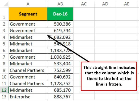
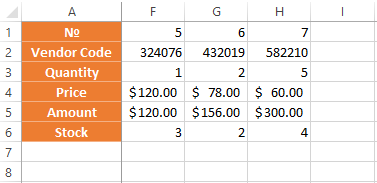
- The first column is frozen. The grey line appears at the end of column A indicating that the column to the left is frozen. The column AB shown in the following image is the last scrolled column of the dataset.

- On scrolling (from left to right) through the remaining columns of the dataset, column A is visible. The same is shown in the following image.

In the same way, the first row can be frozen.
#2 Freeze Multiple Columns in Excel
Freezing multiple excel columns is similar to freezing multiple rows. For freezing multiple columns, select the first right-hand side cell immediately after the last column to be frozen. This is because multiple columns are frozen based on the current selection.
Similarly, for freezing multiple rows, select the first cell immediately below the last row to be frozen.
For example, to freeze the columns A, B, and C, select the cell D1. By freezing the first three columns, they remain visible to the user at all times. Likewise, to freeze the rows 1, 2, and 3, select the cell A4.
The shortcut to freeze multiple excel columns is “Alt+W+F+F” (when pressed one by one).

Let us consider an example.
Example #2
Working on the data of example #1, we want to freeze the first four columns, A, B, C, and D.
The steps for freezing multiple excel columns are listed as follows:
Step 1: Select the cell E1. This is because the first four columns are to be frozen.
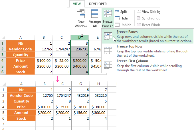
Step 2: In the View tab, click the “freeze panes” drop-down under the “window” section. Select “freeze panes,” as shown in the succeeding image.
Alternatively, press the shortcut keys “Alt+W+F+F” one by one.
Step 3: The first four columns are frozen. The grey line appears (shown in the following image) at the end of column D, indicating that the columns to the left are frozen.
The columns R and S shown in the following image are the scrolled columns towards the end of the dataset.
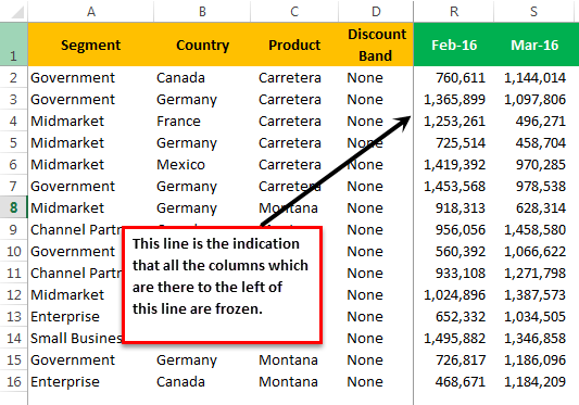
Step 4: On scrolling (from left to right) till the last column of the dataset, the first four columns are visible. The same is shown in the following image.
#3 Freeze the Row and Column Together in Excel
Usually, the first row and the first column of a database contain headers. The user might want to view the row 1 and the column A simultaneously and at all times. Hence, it is essential to lock them together to permit their visibility while scrolling down and from left to right.
The only difference between the methods #2 and #3 is in the selection of the cell (step 1). With the “freeze panes” option, Excel freezes the rows and columns preceding the current active cell.
The shortcut to freeze the row and column together is “Alt+W+F+F” (when pressed one by one).
Let us consider an example.
Example #3
Working on the data of example #1, we want to freeze the first row (row 1) and the first column (column A) at the same time.
The steps to freeze the excel row 1 and column A together are listed as follows:
Step 1: Select the cell B2.
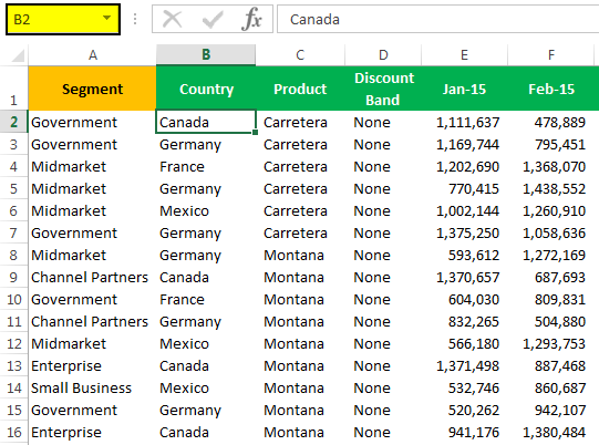
Step 2: Press the shortcut keys “Alt+W+F+F” one by one. It freezes the column to the left of the selected cell B2. At the same time, the row preceding the active cell (B2) is also frozen, as shown in the following image.
Hence two grey lines appear, one at the end of row 1 (horizontal) and the other at the end of column A (vertical).
Note: Alternatively, the “freeze panes” option can be selected from the “freeze panes” drop-down of the View tab.
Step 3: On scrolling from top to bottom and left to right, the row 1 and column A are visible. The same is shown in the following image.
Note: It is possible to freeze as many rows and columns depending on the requirement. The condition is that freezing of multiple excel rows and columns should begin with the top row (row 1) and the first column (column A).
#4 Unfreeze Panes in Excel
Unfreezing of panes does not require any cells to be selected. The steps to unfreeze panes in Excel are listed as follows:
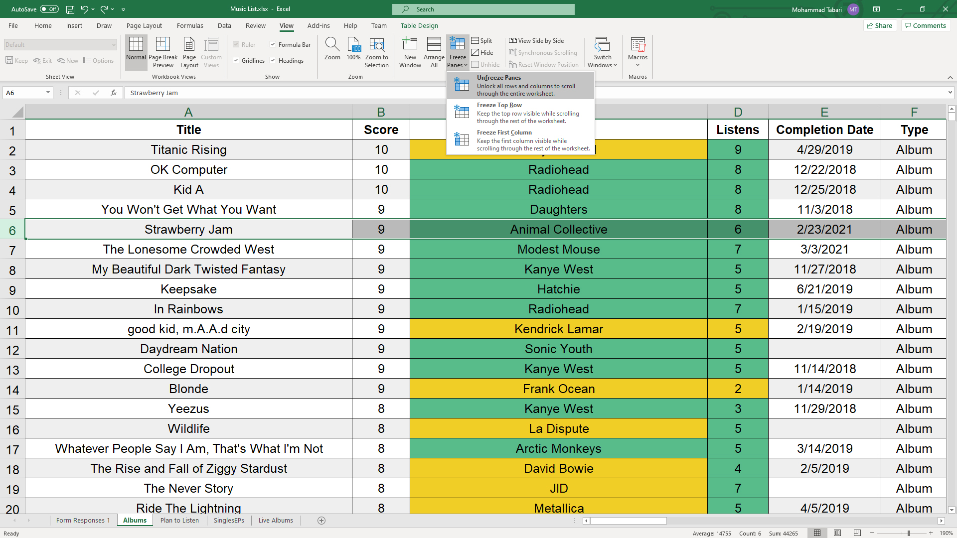
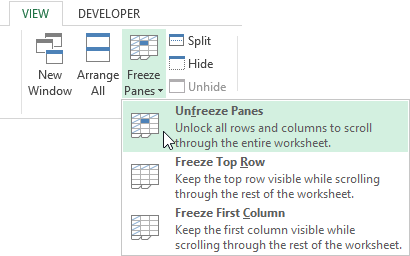
Step 1: In the View tab, click the “freeze panes” drop-down under the “window” section. Select “unfreeze panes,” as shown in the succeeding image.
Alternatively, press the shortcut keys “Alt+W+F+F” one by one.
Step 2: The grey lines are removed, as shown in the following image.
Note: The “unfreeze panes” option appears only after freezes have been applied to the Excel worksheet.
The Rules of Freezing in Excel
The norms governing the freezing of rows and columns are listed as follows:
- It is not possible to freeze excel rows and columns in the middle of the worksheet.
- The option “freeze panes” can be applied only once. It is not possible to create multiple “freeze panes” in a single worksheet.
- The rows and columns to be fixed should be visible at the time of freezing. Otherwise, they will remain hidden even after freezing.
Note 1: To divide a worksheet into two or more areas with separate scroll barsIn Excel, there are two scroll bars: one is a vertical scroll bar that is used to view data from up and down, and the other is a horizontal scroll bar that is used to view data from left to right.read more for each, use the “split” option. This is available in the “window” section of the View tab.
Note 2: To fix the header row of a large dataset that does not fit into the screen, create an Excel tableIn excel, tables are a range with data in rows and columns, and they expand when new data is inserted in the range in any new row or column in the table. To use a table, click on the table and select the data range.read more. Moreover, ensure the visibility of this row by selecting any cell within the table before scrolling.
Frequently Asked Questions
1. What does freezing columns mean and how to freeze the first column in Excel?
Freezing a column means locking it in order to keep it visible while the user scrolls through the database. This is specifically helpful if a column contains headers which are required to be seen at all times.
After freezing, a grey line appears to indicate the frozen columns on its left. The steps to freeze the first column (column A) are listed as follows:
• In the View tab, click the “freeze panes” drop-down under the “window” section.
• Select “freeze first column.” Alternatively, press the shortcut keys “Alt+W+F+C” one by one.
• The first column (column A) is frozen.
Note: For freezing the first row, select “freeze top row” from the “freeze panes” drop-down of the View tab.
2. How to freeze multiple columns in Excel?
Let us freeze columns A, B, C, D, and E. The steps to freeze multiple columns in Excel are listed as follows:
• Select either the column or the first cell to the right of the last column to be frozen (column E). So, select either column F or the cell F1.
• In the View tab, click the “freeze panes” drop-down under the “window” section.
• Select “freeze panes.” Alternatively, press the shortcut keys “Alt+W+F+F” one by one.
• The columns A B, C, D, and E are frozen as indicated by the grey line at the end of column E.
3. How to freeze rows and columns together in Excel?
Let us freeze rows 1, 2, and 3 and columns A, B, and C. The steps to freeze the given rows and columns together are listed as follows:
• Select cell D4 based on the following parameters:
a. It immediately follows the last row to be frozen (row 3).
b. It is to the right of the last column to be frozen (column C).
• In the View tab, click the “freeze panes” drop-down under the “window” section.
• Select “freeze panes.” Alternatively, press the shortcut keys “Alt+W+F+F” one by one.
• The rows 1, 2, and 3 and columns A, B, and C are frozen. This is indicated by the grey line appearing below row 3 and at the end of column C.
Note: The freezing of multiple excel rows and columns should begin with the top row (row 1) and the first column (column A).
Recommended Articles
This has been a guide to freezing columns in Excel. Here we discuss how to freeze the first column, multiple columns, and both rows and columns. For more on Excel, take a look at the following articles-
- Adding Columns in ExcelAdding a column in excel means inserting a new column to the existing dataset.read more
- Group Excel ColumnsIn Excel, grouping one or more columns together in a worksheet is referred to as group column and I t allows you to contract or expand the column.read more
- Column Lock in ExcelThe Column Lock feature in Excel is designed to prevent any mishaps or unwanted modifications in data caused by a user’s mistake. It may be used on single or multiple columns, with cell formatting ranging from locked to unlocked, and the workbook can be password protected.read more
- Column Sort in Excel
I recently helped a friend with Excel, and when I asked him how the spreadsheet looked, he hesitated. Finally, he looked at me and said, “It’s overwhelming.” The data was OK, but he wanted to see the top row when he scrolled. The solution was to show him how to freeze rows and columns in Excel so that key headings or cells were always visible. I’ve outlined four scenarios and solution steps.
This was a good communication lesson for me. It reminded me that we all have different skill levels and vocabularies. For example, when you’re new, you’re probably not thinking in terms like “how to freeze panes in Excel.” You may not know what a pane is. It’s not describing your problem. My friend was thinking in terms of a “sticky header,” or “Excel floating header,” or “pinning rows.” I wasn’t thinking of any of those.
Let’s Start with Excel Panes
An Excel pane is a set of columns and rows defined by cells. You get to determine the size, shape, and location. For many people, it might be the top row. For others, it’s an inverted L-shape and contains the top row and first column. You’re the spreadsheet architect and can define your pane.
Regarding spreadsheets, you can “freeze panes” or “split panes.” Splitting panes is a bit more complex because you have separate windows of your data on the worksheet. So, for the sake of simplicity, this tutorial will cover freezing panes.
If your columns and rows aren’t in the orientation you want, you may want to learn how to transpose or switch columns and rows in Excel.
Why Lock Spreadsheet Cells?
A key benefit to locking or freezing cells is seeing the important information regardless of scrolling. The split pane data stays fixed. Your spreadsheet can contain panes with column headings, multiple rows, multiple columns, or both.
Otherwise, losing focus on a large worksheet is easy when you don’t have column headings or identifiers. I’ve had times where I’ve entered data only to see I was one cell off and produced Excel formula errors. By locking various sections, you have a consistent reference point. This also helps readability.
Typically, the cells you want to stay sticky are labels like headers. However, they could just as easily be an entire column, such as employee names.
Let’s go through four examples and keyboard shortcuts to freeze panes in Excel.
1 – How to Freeze the Top Row
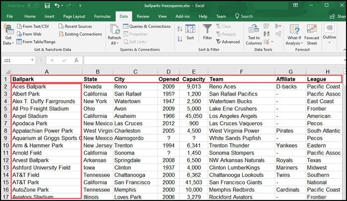
This freeze row example is perhaps the most common because people like to lock the top row that contains headers, such as in the example below.
Another solution is to format the spreadsheet as an Excel table.
- Open your worksheet.
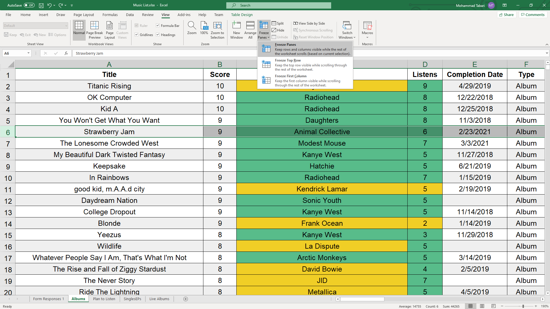
- Click the View tab on the ribbon.
- On the Freeze Panes button, click the small triangle ▼ (drop-down arrow) in the lower right corner. You should see a new menu with three options.

- Click the menu option Freeze Top Row.
- Scroll down your sheet to ensure the first row stays locked at the top.
You should see a darker border under row 1.
Keyboard Shortcut – Lock Top Row
I like to do this shortcut slowly the first time to see the ALT key letter assignments as you type. I can see the keyboard assignments in the example below once I hit my Alt key. Some people prefer to add the Freeze Panes command to the Quick Access toolbar because they frequently use it.

Alt + w + f + r
2 – How to Freeze the First Column
A similar scenario is when you want to freeze the leftmost column. I guess Microsoft researched this to determine the most common sub-menu options.
I find this option helpful when I have a spreadsheet with many columns and I need to fill in data without using an Excel data form.

- Open your Excel worksheet.
- Click the View tab on the ribbon.
- On the Freeze Panes button, click the small triangle ▼. You should see a new menu with your 3 options.
- Click the option Freeze First Column.
- Scroll across your sheet to make sure the left column stays fixed.
Keyboard Shortcut – Lock First Column
Alt + w + f + c
3 – How to Freeze the Top Row & First Column
This is my favorite option. If you look at Microsoft’s initial Freeze Panes options, there isn’t one for the top row and first column. Instead, we’ll use the generic option called Freeze Panes.
The subtext reads, “Keep rows and columns visible while the rest of the worksheet scrolls (based on current selection).” Some folks get confused as they think they have to highlight data to make a selection.
Instead, consider the selection of the first cell outside your fixed column and row. If I wanted to lock the top row and top column, that selection cell would be cell B2 or Nevada. Regardless of whether I scroll down or to the right, the first cell that disappears when I scroll is B2.

- Open your Excel spreadsheet.
- Click cell B2. (Your set cell.)
- Click the View tab on the ribbon.
- On the Freeze Panes button, click the small triangle ▼ in the lower right corner. You should see a dropdown menu with your 3 options.
- Click the option Freeze Panes.
- Scroll down your worksheet to make sure the first row stays at the top.
- Scroll across your sheet to make sure your first column stays locked on the left.
Keyboard Shortcut – Freeze Panes
Alt + w + f + f
4 – Freeze Multiple Columns or Rows
On occasion, I get some Excel worksheets where the author puts descriptive text above the data. My header isn’t in Row 1 but further down in Row 5. Or I want to lock multiple columns to the left. In the example below, I want to lock Columns A & B and Rows 1-5.

The process is the same, I just need to click the set cell that stops the fixed area. In this case, it would be cell C6 or “Regions Field.” The content above and to the left is frozen.
Everything in the red boxes would be locked. The downside is you may give up much of the screen real estate.
Why Freeze Panes May Not Work
There are some rules surrounding this feature. If you don’t follow these, freeze panes may not work.
Quick test: If you type Ctrl + Home and your cursor moves to cell A1, you haven’t locked anything.
- If you dislike your settings, use the Unfreeze Panes command.
- This feature won’t work on a protected worksheet or Page Layout View.
- If you’re editing a value in the Formula bar, the View menu will be disabled.
If you need to see the same header on printed pages, Microsoft has instructions.
As you’ve seen, choosing what content to freeze is easy. You can freeze the top row, first column, both, or a subset of your data, depending on what you want to do with it. The flexibility is part of what makes Microsoft Excel such an excellent program for organizing and analyzing information from any field.
When you’re working with a lot of spreadsheet data on your laptop, keeping track of everything can be difficult. It’s one thing to compare one or two rows of information when dealing with a small subset of data, but when a dozen rows are involved, things get unwieldy. And we haven’t even started talking about columns yet. When your spreadsheets become unmanageable, there’s only one solution: freeze the rows and columns.
Freezing rows and columns in Excel makes navigating your spreadsheet much easier. When done correctly, the chosen panes are locked in place; this means those specific rows are always visible, no matter how far you scroll down. More often than not, you’ll only freeze a couple of rows or a column, but Excel doesn’t limit how many of either you can freeze, which can come in handy for larger sheets.
This how-to works with Microsoft Excel 2016 as well as later versions. However, the this method also works with Google Sheets, OpenOffice and LibreOffice. Ready to get to work? Here’s how to freeze rows and columns in Excel:
- More: How to put Windows 10 into Safe Mode
- Here’s how to lock cells in Excel and how to recover a deleted or unsaved file in Excel
- This is how to use VLOOKUP in Excel and add additional rows above or below in Excel
How to freeze a row in Excel
1. Select the row right below the row or rows you want to freeze. If you want to freeze columns, select the cell immediately to the right of the column you want to freeze. In this example, we want to freeze rows 1 to 5, so we’ve selected row 6.
2. Go to the View tab. This is located at the very top, inbetween «Review» and «Add-ins.»
3. Select the Freeze Panes option and click «Freeze Panes.» This selection can be found in the same place where «New Window» and «Arrange All» are located.
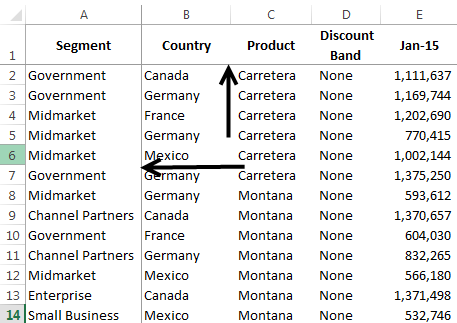
That’s all there is to it. As you can see in our example, the frozen rows will stay visible when you scroll down. You can tell where the rows were frozen by the green line dividing the frozen rows and the rows below them.
If you want to unfreeze the rows, go back to the Freeze Panes command and choose «Unfreeze Panes».
Note that under the Freeze Panes command, you can also choose «Freeze Top Row,» which will freeze the top row that’s visible (and any others above it) or «Freeze First Column,» which will keep the leftmost column visible when you scroll horizontally.
Besides allowing you to compare different rows in a long spreadsheet, the freeze panes feature lets you keep important information, such as table headings, always in view.
Need more Excel tricks? Check out our tutorials on How to Lock Cells in Excel and How to Use VLOOKUP in Excel.
Get instant access to breaking news, the hottest reviews, great deals and helpful tips.
![]()
Download Article
![]()
Download Article
- Freezing the First Column or Row
- Freezing Multiple Columns or Rows
- Video
- Q&A
|
|
|
This wikiHow teaches you how to freeze specific rows and columns in your Microsoft Excel worksheet. Freezing rows or columns ensures that certain cells remain visible as you scroll through the data. If you want to easily edit two parts of the spreadsheet at once, splitting your panes will make the task much easier.
-
1
Click the View tab. It’s at the top of Excel. Frozen cells are rows or columns that remain visible while you scroll through a worksheet.[1]
If you want column headers or row labels to remain visible as you work with large amounts of data, you’ll likely find it helpful to lock those cells into place.- Only whole rows or columns can be frozen. It is not possible to freeze individual cells.
-
2
Click the Freeze Panes button. It’s in the «Window» section of the toolbar. A set of three freezing options will appear.
Advertisement
-
3
Click Freeze Top Row or Freeze First Column. If you want to keep the top row of cells in place as you scroll down through your data, select Freeze Top Row. To keep the first column in place as you scroll horizontally, select Freeze First Column.
-
4
Unfreeze your cells. If you want to unlock the frozen cells, click the Freeze Panes menu again and select Unfreeze Panes.


Advertisement
-
1
Select the row or column after those you want to freeze. If the data you want to keep stationary takes up more than one row or column, click the column letter or row number after those you want to freeze. For example:
- If you want to keep rows 1, 2, and 3 in place as you scroll down through your data, click row 4 to select it.
- If you want columns A and B to remain still as you scroll sideways through your data, click column C to select it.
- Frozen cells must connect to the top or left edge of the spreadsheet. It’s not possible to freeze rows or columns in the middle of the sheet.[2]
-
2
Click the View tab. It’s at the top of Excel.
-
3
Click the Freeze Panes button. It’s in the «Window» section of the toolbar. A set of three freezing options will appear.
-
4
Click Freeze Panes on the menu. It’s at the top of the menu. This freezes the columns or rows before the one you selected.
-
5
Unfreeze your cells. If you want to unlock the frozen cells, click the Freeze Panes menu again and select Unfreeze Panes.


Advertisement
Add New Question
-
Question
How do I freeze the top two rows?

Select the row directly under the rows you want to freeze (in this case, the third row). Go to View, Freeze Panes, and select «Freeze Panes.» Everything above the row you have selected will be frozen.
Ask a Question
200 characters left
Include your email address to get a message when this question is answered.
Submit
Advertisement
Thanks for submitting a tip for review!
wikiHow Video: How to Freeze Cells in Excel
About This Article
Article SummaryX
1. Click View.
2. Click Freeze Panes.
3. Select Freeze Top Row or Freeze First Column.
Did this summary help you?
Thanks to all authors for creating a page that has been read 171,421 times.
Is this article up to date?
The Microsoft Excel program is designed not only to enter data into the table conveniently and edit it as you need it, but also to view large blocks of information. Most people using PCs work with it constantly.
The columns and rows names can be significantly removed from the cells with which the user is working at this time. Scrolling the page to see the name of the document is not comfortable for any user. Therefore, the Tabular Processor has possibilities to fix certain areas.
Locking a row in Excel while scrolling
Usually an Excel table has one cap. Meanwhile, this document can have up to thousands of rows. Working with multipage table blocks is inconvenient when column names are not visible. Scrolling the page to its beginning to return to the correct cell is absolutely irrational. To make the cap visible when scrolling, fix the top row of the Excel table, following these actions:
- Create the needed table and fill it with the data.
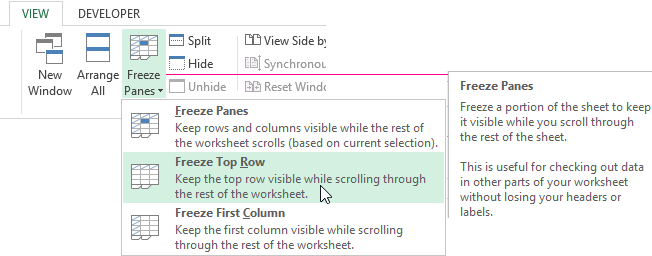
- Make any of the cells active. Go to the “VIEW” tab using the tool “Freeze Panes”.
- In the menu select the “Freeze Top Row” functions.
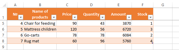
You will get a delimiting line under the top line. Now when you scroll vertically the table cap will be always visible.
Locking several rows in Excel while scrolling
Let us suppose, a user needs to fix not only the cap. For instance, another row or even a couple of rows must be fixed when scrolling the document. Doing it is possible and easy, when you follow these steps:
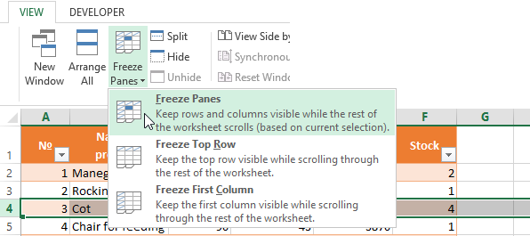
- Select any cell under the line, which we will fix. This action will help Excel to “understand”, which area should be fixed;
- Now select the “Freeze Panes” tool.
When you perform horizontal and vertical scrolling, the cap and the top row of the table remain fixed. Thus, you can fix two, three, four and more rows.
Note: This method works for 2007 and 2010 Excel versions. In earlier versions the “Lock areas” tool is located in the “Window” menu on the main page. There you must always (!) activate the cell under the freeze row.
Freezing columns in Excel
For instance, the information in the table has a horizontal direction. It is not concentrated in columns, but located in rows. For his comfort, the user must freeze the first column, containing the lines’ names in horizontal scrolling.
- Select any cell of the chosen table so that Excel understands with what data it will work. Pin the first column in the menu you will see..
- Now, when the document is scrolled to the right horizontally, the needed column will be fixed.
To freeze several columns, select the cell at the page bottom (to the right from the fixed column). Pick the “Freeze Panes” button.
How to freeze the row and column in Excel
You have a task – to freeze the selected area, which contains two columns and two rows.
Make a cell at the intersection of the fixed rows and columns active. However, the cell must be not placed in the fixed area. It should have the position right under the required lines (to the right of the required columns). Pick the first option in Excel Locking Areas. The photo shows that when scrolling, the selected areas remain at the same place.
Removing a fixed area in Excel
After fixing a row or a column of the table the button deleting all pivot tables becomes available.
After clicking – «Unfreeze Panes», all the locked areas of the worksheet become unlocked.
With Excel it’s often quite convenient to freeze part of your spreadsheet and keep it visible at all time. Typically, freezing the top rows of left columns of your Excel spreadsheet allows you to scroll down but keep an eye on the headers.
This result can be achieved by freezing panes. Panes can be recognied by a grey vertical or horizontal line.
How to freeze panes in Excel
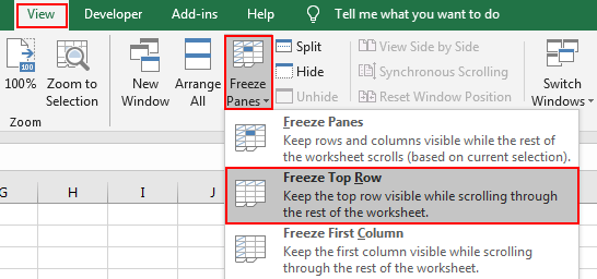
To freeze the 1st row, go in the «View» tab, click «Freeze Panes» and then «Freeze Top Row».

To freeze the 1st column, go in the «View» tab, click «Freeze Panes» and then «Freeze First Column».

You can also freeze multiple rows, multiple columns, or a combination of any number of rows and columns. To do so:
-
Select the first row that you don’t need to keep visible. For instance if you want to freeze columns A to D, select any cell in column E. If you want to freeze rows 1 to 3, select any cell in row 4. And if you want to freeze columns A to D AND rows 1 to 3, select cell E4.
-
Go in the «View» tab, click «Freeze Panes» and then «Freeze Panes».

Note: when you freeze panes, the areas on the top or left of your spreadsheet are really frozen. If you scroll, they will always remain visible. If you would like to be able to scroll in the frozen area, what you need it is to Split panes, as explained below.
How to unfreeze panes in Excel
Go to the «View» tab, click «Freeze Panes» and then «Unfreeze Panes».

How to split a worksheet in Excel
While freezing panes allows you to freeze an area located at the top or left of your spreadsheet, you may want a different behavior and be allowed to scroll within each of the separated parts of the worksheet.
For this you need not to freeze but to split your worksheet. It works exactly like freezing panes, but instead go to the «View» tab, and click «Split».

The areas delimited are not frozen and you can scroll in each of them separately. Contrary to frozen panes, you can also drag and drop the pane to move it to a different row or column.
To unsplit, just click again on the «Split» button.
Suppose we create a large table in excel spreadsheet and it lists large amount of data. There are headers in the first row, and if we want to drag the scroll bar to view the bottom of table, the headers are hidden due to it lists on the top. So, in this case if we want to see the headers all the time, we need to freeze the first row to make it fixed and always displays on the top even we drag the scrollbar. On the other side, sometimes we need to freeze more rows, or columns, or even freeze row and column simultaneously. To implement this, we need to know the way to freeze row and columns. This article will introduce different ways to freeze row and columns with examples for you, you can’t miss it.
Table of Contents
- Method 1: How to Freeze the First Row in Excel Spreadsheet
- Method 2: How to Freeze Multiple Rows in Excel Spreadsheet
- Method 3: How to Freeze the First Column in Excel Spreadsheet
- Method 4: How to Freeze Row and Column in Excel Spreadsheet
- Method 5: How to Freeze Rows and Columns in Excel Spreadsheet
Method 1: How to Freeze the First Row in Excel Spreadsheet
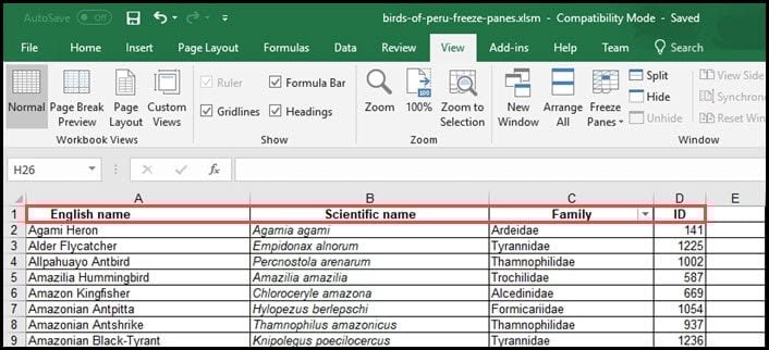
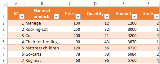
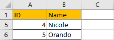
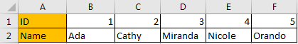
In most daily work, freeze the first row in table is frequently needed due to in most tables the first row lists the headers. So, people always want to see the headers on top no matter whether they drag the scrollbar to the end or not. See example below:
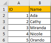
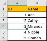
Suppose it lists a long list of ID and names. Header ID and Name are listed on the top. Now let’s freeze the first row.
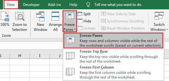
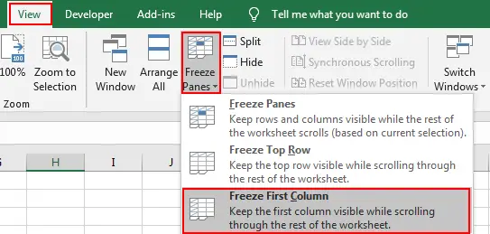
Step 1: Click View in the ribbon, then click Freeze Panes in Window group, then click the small triangle of Freeze Panes to load below three options, select the middle one ‘Freeze Top Row’.
Step 2: After above operating. The first top row is fixed and always displayed on the top. Try to drag the scrollbar. You can see the header row is stayed on the top.
Method 2: How to Freeze Multiple Rows in Excel Spreadsheet
If you want to freeze the first three rows in excel, you can just select the first cell in the fourth row, then freeze the rows above the selected cell. See details below.
Step 1: Click A4 in the table.
Step 2: Click View in the ribbon, then click Freeze Panes in Window group, then click the small triangle of Freeze Panes to load below three options, select the first one ‘Freeze Panes’.
Step 3: Try to drag the scrollbar. Verify that top three rows are fixed.
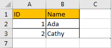
Method 3: How to Freeze the First Column in Excel Spreadsheet
See screenshot below:
Now let’s freeze the first column. The way is similar with freeze the first row.
Step 1: Click View in the ribbon, then click Freeze Panes in Window group, then click the small triangle of Freeze Panes to load below three options, select the middle one ‘Freeze First Column’.
Step 2: Verify if it works well.
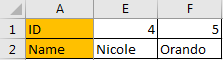
Obviously, it works.
Method 4: How to Freeze Row and Column in Excel Spreadsheet
If you want to just freeze the first row and column, just click on B2. Then click View->Freeze Panes->Freeze Panes in Window group.

Method 5: How to Freeze Rows and Columns in Excel Spreadsheet
If you want to freeze multiple rows and columns, refer to the description of Freeze Panes ‘Keep rows and column visible while the rest of the worksheet scrolls (based on current selection)’ we can know that we can select a cell to make it as the first cell outside of your fixed area. For example, if we want to freeze the top three rows and first two columns (row 4 is not fixed and column C is not fixed), we can click on C4, then repeat above steps to freeze panes.
Wow, so much confusion.
Raystafarian and Tog are correct and Siva Charan is utterly wrong in his statement leading off his answer: You can’t do only specific column.
To word things better all around, consider the following:
-
You can freeze only columns if desired. One or more, frozen to the left of the working area. If you select the row 1 cell of the first column to the right of the one you want frozen and freeze, the that column to the left of the selected cell, and all to its left, are in the frozen section, but all rows scroll. This seems to be what the question asked. More though later.
-
You can freeze only rows if desired. One or more, frozen above the working area. If you select the column A cell of the first row below the one you want frozen and freeze, the that row above the selected cell, and all above it, are in the frozen section, but all columns scroll.
-
Select some cell «in the grid», perhaps f10, and freeze, and like in 1. and 2. above, rows above it and columns to the left of it freeze. This is what
Siva Charanwas talking about, but he was flat wrong in saying «You can’t do only specific column.» More on this too, later.
In each case, rows above and columns to the left of the selected cell were frozen. In 1., above, there were NO rows above, so the effect is of only columns being frozen. In 2., above, there are NO columns to the left, so the effect is of only rows being frozen. So it is the same concept in ALL cases applied to the specifics of your selected cell.
Intriguingly, if one selects A1 and presses Alt-W-F-F, the screen «quarters» with the usual «freeze marks» (a dark black line on the lower and right borders of cells that are frozen makes a cross on the screen). The lower right quadrant is scrollable as if one had selected its upper leftmost cell and frozen panes.
However, and this may be what Siva Charan understood the question to be asking, you cannot have, say, columns A, B, C, D, E, and F as your working area and freeze ONLY column B, say. It would be columns A and B: column B and all columns to its left.
You can, though, move the grid about until column B is the leftmost column viewed on the screen and then freeze it. Both columns A and B would again be frozen, but since ONLY column B appears on the screen, it would seem like you had frozen only column B. So you can get some of the effect of that, but not the actuality. If you want column H, perhaps, frozen with work areas to the left and right, you need to do something else altogether.
So, Malachi‘s answer comes into play. He discusses SPLITTING the window into two parts. In that case, you have much the same results as with freezing panes, but there are differences. Not enough differences to freeze a column in the middle of the screen and work in both the left of it and the right of it, but differences.
The main purpose of Splitting is to have two different areas you want to work WITH and for them to both be scrollable. Perhaps you have entries on line 4 that relate to entries on line 404 and you want to view both lines at once, be able to move between those rows without going up or down 400 lines each time, and maybe even then scroll down one line in each to do work in lines 5 and 405.
Freezing panes is mostly to keep titles on the screen, so that, unlike almost every website table you ever encounter, you always know what a column is supposed to be even if you scroll four feet down in it. So you work in one area and use the frozen area for reference. Only the work area needs scrolling. Splitting’s purpose is more to keep both areas in view and be able to work in both areas. And then to scroll for further work. However, the scrolling is manual. You must do both areas, there being no automatic synchronization.
A third thing that does these kinds of things is in that same piece of the Ribbon Menu system. It is New Window. It opens an entirely new window for the file, complete with its own Ribbon Menu system. The first window title (green bar at the top of the window changes from, say, Book1 - Excel to Book1 - 1 - Excel and the new one has a «2» in the middle. Pay attention to those by the way, as when you close them, you want to close the extra windows (not the «1» window), then close from the remaining one or some oddities can happen. Nothing harmful, just annoying, but still… If you have macros that might close the file, keep this thought in the front of your head.
The fun thing about new windows is that:
-
Can be set to scroll synchronously, so you can see, say, twenty columns at the left of a table, then a window with columns 97-112 perhaps in the other, ignoring the 77 columns in between without dropping little dukies like Hiding those columns and forgetting to unhide them when saving, and not having access to them either if you need the odd look at something in them. Or not synchronously if preferred for your use.
-
You can size the windows and arrange them on your monitor or monitors as desired. So if you want column AF to be a single column in the center of your screen with a view of columns to its left and to its right to either side of it, you can just open two windows so you have three altogether and arrange and size the windows to do just that. Column AF’s window, tall and narrow, in the middle of your screen and the other two windows on each side of it perhaps filling the monitor’s screen. Or maybe you drink Bill(ionaire) Gates’ Kool-Aid and love little windows all over your screen. It’s all good. If you set the middle window (column AF) to not scroll synchronously, it remains effectively frozen there as you work.
So three solid and oft used features to try to accomplish whatever is truly asked here. By the way, «back in the day» when this was asked (2012) Excel was still MDI so the new windows would have ALL stayed in the program’s work area and would not have had their own Ribbon Menu systems taking up space. It was common then to pop out four of them each taking up a quarter of the work area. Or cascaded, but the approaches solved two different problems so one was not «better» than the other even though people sure argued the point!
Last thought since this involves at least tangentially the idea of how to get screen space to do what one needs: IF you have two or more monitors, and set Windows correctly, you can un-Maximize your Excel window (or any program that allows you to control its window size), pull its edges manually to fill the screen again, then take the appropriate border and drag it ONTO THE OTHER MONITOR. So two monitors, left and right, programs load on the left one? Do that, dragging the right edge of the screen-sized window onto the right monitor even all the way to its far edge and you have probably 50+ columns showing. More or less as one’s column widths dictate, and of course, as one’s monitors dictate. The monitors do not even have to be the same size. So you need to read a three foot wide column? No problema! Just read it on screen! No entering the cell and doing it the hard way. Always needed 65 columns but hated scaling down to 50% magnification? No problema! And it will remember the sizing too (Well, as much as Windows permits… notice your dialog boxes shift about for no obvious reason sometimes? That’s Windows jacking you.) and launch that way the next time. I have different size monitors, by the way, so I speak from experience.
I’d tell you how to get more than three lines in the formula editor too (it’s incredibly simple and annoying obvious once you know it, hard to imagine you worked 30 years with Excel before noticing it…), but can’t figure a way that that would even tangentially touch on the question’s subject.
Aw heck, why not? Someone can chop it out if it doth offend their sensibilities.
Clock in the formula editor (or press F2). Click the little arrow on the right to expand it (don’t have to, I just always like knowing I can leave it as a single line when exiting it). Look at the column headers underneath it. Notice the VERY ODD fact that the top[ third or so of the gray area they are in is empty? The column division lines don’t run fully top to bottom, just fill the bottom two-thirds. The column letter labels are consistent with that. So there’s this one-third height of gray that doesn’t precisely seem to be part of them, but you don’t really notice until you look closely and think «Wha…?»
If you put your cursor in the editing area, then move it slowly down toward the letters, the I-beam pointer suddenly turns into a standard vertical double headed pointer. Just over halfway on the I-beam as it moves down into the gray.
Halt! The moment you have the vertical double headed pointer, you can click on the mouse and drag it down. As many lines in the editor as you like, until you reach the bottom of the screen. My boss has a 60″ monitor above two 32″ monitors and when I show him, we used the 60″ monitor and had 80 or so lines. No more scrolling around in a formula just to view a piece of it!
Helpful too, for viewing lengthy cell content with F2, quicker than the two monitor-wide thing above if one needs it infrequently or doesn’t wish to devote two monitors to Excel.
Be SURE to restore it to the standard three lines (or five, my new standard) or it could be a little unexpected when you press F2! As «unexpected» it might even cover something you needed to see for the current edit which would layer in even more annoyance. Otherwise though, especially when using LET() or IFS() the extra space can let you keep easy track of all elements.
I’ve begun laying out formulas like a programmer can, breaking lines for clarity, making them much more readable. So a simple use might see LET() with the first line containing elements that have references or values in them that might be changed by a user, then another one (or several lines) with further elements derived from them, and I like to do that as line 2 elements deriving directly from the line 1 elements, and line 3 for elements using anything in lines 1 or 2, etc., then a blank line, then the working part of the formula, and finish off with the final «)» on its own line. Indenting at the left to keep everything in proper related groupings. Set up a 25 IF IFS() as one line for each IF and it not only becomes incredibly readable, but if the statements are similar, ANY oddity like a dropped comma stands out. Adding spaces after a parameter’s comma in functions makes them much more easily edited or understood as well.
It’s hugely freeing to not have to stuff everything right smack up against each other to try to minimize the need to scroll if reading or editing it. Dense packed formulas are incredibly hard to fix for changes and for when a comma is dropped and you have to figure out where.
Well, that’s it though, just clearing up the three ways to «freeze» (essentially) parts of your screen for better working with your spreadsheets.