Free cells in excel

How to Freeze Cells in Excel? (with Examples)

Freezing cells in Excel means that when we move down to the data or move up the cells, it freezes the cells displayed on the window. To freeze cells in Excel, we must select those cells we want to freeze. Then, in the “View” tab in the windows section, click on “Freeze Panes” and again click on “Freeze Panes” from the drop-down list. As a result, this will freeze the selected cells. First, let us understand how to freeze rows and columns in Excel by a simple example.

You can download this Freeze Rows and Columns Excel Cell template here – Freeze Rows and Columns Excel Cell template

How to Freeze Cells in Excel? (with Examples)
- Example #1
- Example #2
- Use of Rows & Column Freezing in Excel Cell
- Things to Remember
- Recommended Articles

Example #1

Freezing the Rows: Given below is a simple example of a calendar.

We must first select the row which we need to freeze the cell by clicking on the number of the row.
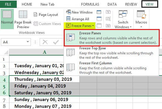
Then, click on the “View” tab on the ribbon. Next, we must select the “Freeze Panes” command on the “View” tab.
The selected rows get frozen in their position, and a grey line denotes it. We can scroll down the entire worksheet and continue viewing the frozen rows at the top. As we can see in the snapshot below, the rows above the grey line are frozen and do not move after we scroll the worksheet.
We can repeat the same process for unfreezing the cells. Once we have frozen the cells, the same command is changed in the “View” tab. The “Freeze Panes” in the Excel command is now changed to the “Unfreeze Panes” command. By clicking on it, the frozen cells are unfrozen. This command unlocks all the rows and columns to scroll through the worksheet.

The date is provided in the columns instead of the rows in this example.

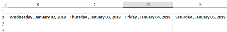
Step 1: We need to select the columns, which we need to freeze Excel cells by clicking on the alphabet of the column.

Step 2: After selecting the columns, we need to click on the “View” tab on the ribbon. Then, we need to choose the “Freeze Panes” command on the “View” tab.

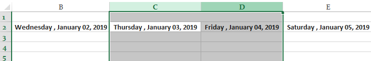
Step 3: The selected columns get frozen in their position, and a grey line denotes it. We can scroll the entire worksheet and continue viewing the frozen columns. As we can see in the snapshot below, the columns beside the grey line are frozen and do not move after we scroll the worksheet.

For unfreezing the columns, we must use the same process as we did in the case of rows by using the “Unfreeze Panes” command from the “View” tab. In addition, there are two other commands in the “Freeze Panes” options: “Freeze Top Row” and “Freeze First Column.”

These commands are used only for freezing the top row and the first column, respectively. For example, the “Freeze Top Row” command freezes the row number “1,” and the “Freeze First Column” command freezes the column number A cell. It is to be noted that we can also freeze rows and columns together. In addition, It is not necessary to lock only the row or the column at a single instance.

Example #2

Let us take an example of the same.

Step 1: The sheet below shows the timesheet of a company. The columns contain the headers as “Day,” “Date,” “Regular Hours,” “Overtime Hours,” “Sick,” “Vacation,” and “Total.”

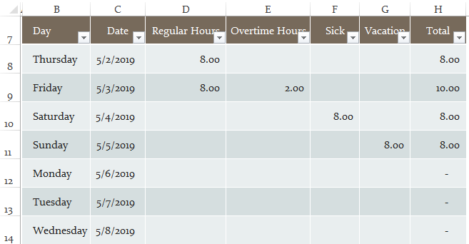
Step 2: We need to see columns “B” and row 7 throughout the worksheet. We have to select the cell above, besides which we need to freeze the columns and rows cells, respectively. In our example, we have to choose the cell number H4.

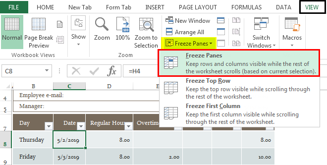
Step 3: After selecting the cell, we need to click on the “View” tab on the ribbon and select the “Freeze Panes” command on the “View” tab.

Step 4: As we can see from the snapshot below, two grey lines denote the locking of cells.

Use of Rows & Column Freezing in Excel Cell

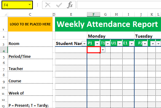
If we use the “Freeze Panes” command to freeze the columns and rows of Excel cells, they will remain displayed on the screen regardless of the magnification settings that we select or how we scroll through the cells. Let us take a practical example of the weekly attendance report of a class.

Step 1: Now, if we take a look at the snapshot below, the rows and columns display various pieces of information such as “Student name,” “Name of the days,” “Room,” etc. The topmost column shows the “logo to be placed here” and the “Weekly Attendance Report.”

In this case, it becomes necessary to freeze certain Excel columns and rows of cells to understand the attendance of the reports. Otherwise, the report becomes vague and difficult to understand.

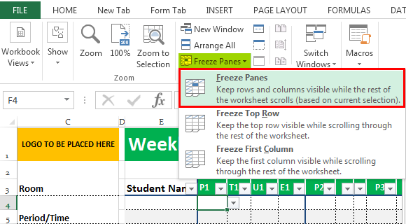
Step 2: We must select the cell at the F4 location as we need to freeze down the rows up to the subject code P1, T1, U1, E1, and columns up to the “Student Name.”

Step 3: Once we select the cell, we must use the “Freeze Panes” command, freezing the cells at the position indicating a grey line.

As a result, we can see that the rows and columns beside and above the selected cell have been frozen, as shown in the snapshots below.

Similarly, we can use the “Unfreeze Panes” command from the “View” tab to unlock the cells which we have frozen.

Hence, explaining the examples above, we used the freezing of rows and columns in Excel.

Things to Remember

When we press the “Ctrl+Home” Excel Shortcut keysAn Excel shortcut is a technique of performing a manual task in a quicker way.read more after giving the “Frozen Panes” command in a worksheet, instead of positioning the cell cursor in cell A1 as normal, Excel sets the cell cursor in the first unfrozen cell.
The “Freeze Panes” in the worksheet cell display consist of a feature for printing a spreadsheet known as “Print Titles.” When we use Print TitlesIn Excel, Print Titles is a feature that lets the users print specific row & column headings on every page of a multi-page report. You need to select “Print Titles” in the Page Layout Tab & enter the required details to perform the function. read more in a report, the columns and rows that we define as the titles are printed at the top and to the left of all data on each report page.
The shortcut keys that get random access to the “Freezing Panes” command are “Alt+W+F.”
In the case of freezing Excel rows and columns together, we must select the cell above, and the rows and columns need to be frozen. We do not have to select the entire row and column together for locking.

wikiHow Video: How to Freeze Cells in Excel

About This Article

Article SummaryX

1. Click View.
2. Click Freeze Panes.
3. Select Freeze Top Row or Freeze First Column.

Did this summary help you?

Thanks to all authors for creating a page that has been read 171,421 times.

Is this article up to date?

Источник

Just assume you are school teacher and have around 90 students in a class which is divided into various sections. Now, you have to collate their marks in every subject in an excel.

If you are using a 15-inch laptop to do this, then as soon as you go to the 25^th row or later you lose the context of which column is for which subject. All of this happens because your header or first row is not fixed and keeps changing as you scroll down. But don’t worry we are here to help you out. 🙂

In this post we are going to help you on how to freeze rows or columns in excel. Freeing in excel will turn some cells (rows and / or columns) to be stagnant and these cells would not change if you move left or right or scroll up or down. There are various ways to freeze cells in excel.

We have listed all the methods below, if you do not want to go through the entire post then you may directly click on the type of excel freeze option you are looking for:

Freeze First Row
Freeze First Column
Freeze Panes
1. Freeze Multiple Rows
2. Freeze Multiple Columns
3. Freeze Rows & Columns at same time

Along with helping you on how to freeze in excel, we will also help you to unfreeze and troubleshooting issues that you might encounter:

Unfreeze Panes
Freeze panes versus Splitting Panes
Freeze Pane is Disabled

Freeze First Row

This feature could be used to freeze a particular row or header that you would need to refer every time while working on excel. In this option only the top row will freeze.

Open the sheet where in you want to freeze any row / header, as an example we would like to freeze the top row highlighted in yellow

Now, navigate to the “View” tab in the Excel Ribbon as shown in above image
Click on the “Freeze Panes” button

Select “Freeze Top Row” option

If you would like to freeze any other row, then scroll down and make that row appear as first in your sheet and then repeat Step 2 to 4.

That’s it. You are all set now. As seen in above image you can now scroll to any corner of the page and you would see that the top row remains intact all the time without any change.

Please note that this option works as long as first row in excel is the one that you really want to freeze. If you have scrolled in the middle of the sheet and Row 30 is appearing as first row, then this option would freeze Row 30 and not Row 1.

Additionally, if you are geek and would like to do it directly using a keyboard shortcut, then please press “Alt + W” followed by “F” and then “R”. Please note that this is not an in-built shortcut, rather it’s the same thing from keyboard as we do from mouse.

Freeze First Column

This feature could be used to freeze a particular column that you would need to refer while working on excel. In this option only the first column will freeze.

Open the sheet where in you want to freeze the column, as an example we would like to freeze the column A – Product

Now, navigate to the “View” tab in the Excel Ribbon as shown in above image
Click on the “Freeze Panes” button

Select “Freeze First Column” option

If you would like to freeze any other column, then move right or left and make that column appear as first in your sheet and then repeat Step 2 to 4.

That’s it. You are all set now. As seen in above image you can now move to most right corner of the page and you would see that the first column sticks there. Please note that this option works as long as first column in excel is the one that you really want to freeze. If you have shifted right in the middle of the sheet and Column M is appearing as first row, then this option would freeze Column M and not Column A.

If you would like to do it directly using a keyboard shortcut, then please press “Alt + W” followed by “F” and then “C”. Please note that this is not an in-built shortcut, rather it’s the same thing from keyboard as we do from mouse.

Freeze Panes

This feature could be used to freeze multiple rows, columns or both at the same time. However, this could be done only for the consecutive rows or columns.

Freeze Panes – Multiple Rows

Open the sheet where in you want to freeze the multiple rows, keep the first row on top and click after the last row till where you want to freeze, as an example we would like to freeze from Row 1 to Row 13 so we will click on Row 14

Now, navigate to the “View” tab in the Excel Ribbon as shown in above image
Click on the “Freeze Panes” button

Select “Freeze Panes” option

That’s it. You are all set now. As seen in above image you can now scroll down and Row 1 to Row 13 will be kept intact without any changes. You can select the range of rows from middle as well like – Row 13 to Row 30, however to do so you will have to ensure that you scroll up and keep Row 13 as your first row in the sheet and repeat the steps listed above. However, be careful as doing so some of your rows (i.e. the ones before Row 13) will be hidden.

Freeze Panes – Multiple Columns

Open the sheet where in you want to freeze the multiple columns, keep the first column to the left and click next to the last column till where you want to freeze, as an example we would like to freeze from Column A to E, so we will click on Column F

Now, navigate to the “View” tab in the Excel Ribbon as shown in above image
Click on the “Freeze Panes” button

Select “Freeze Panes” option

That’s it. You are all set now. As seen in above image you can now move towards right and Column A to E will be kept intact without any changes. You can select the range of columns from middle as well like – Column F to Column L, however to do so you will have to ensure that you move to the left and keep Column F as your first column in the sheet and repeat the steps listed above. However, be careful as doing so some of your columns (i.e. the ones before Column E) will be hidden.

Freeze Panes – Multiple Rows and Columns both

If you have followed the post till now, then you would have already figured out how this has to be done. Yes, you are right we are going to club both the above listed approaches here. Follow us below:

Open the sheet where in you want to freeze the multiple rows and columns, keep the first row on top and first column to the left then click next to the cell of the last column and row till where you want to freeze, as an example we would like to freeze from Row 1 to 13 and Column A to E, so we will click on Cell F14

Now, navigate to the “View” tab in the Excel Ribbon as shown in above image
Click on the “Freeze Panes” button

Select “Freeze Panes” option

That’s it. You are all set now. As seen in above image you can now scroll down and Row 1 to 13 will remain intact and likewise you can move towards right and Column A to E will be kept intact without any changes. You can select the range of columns from middle as well like – Row 17 to 27 and Column F to L, however to do so you will have to ensure that you scroll up and keep Row 17 as your first row and keep Column F as your first column in the sheet and repeat the steps listed above. Be careful here as rows before Row 17 and columns before column F will be hidden.

Unfreeze Panes:

If you have frozen the wrong rows and columns, then you could easily undo it by using “Unfreeze Panes” option. This would remove all the frozen rows and or columns in your excel. This will also work if you have received the sheet from someone else and you are not able to see all the rows and columns despite of removing all filters and unhiding rows columns. To unfreeze panes –

Open the sheet wherein you want to unfreeze rows and or columns
Now, navigate to the “View” tab in the Excel Ribbon
Click on the “Freeze Panes” button

Select “Unfreeze Panes” option as shown above

With this all the rows and or columns would unfreeze, as shown in above image. Please note that you would not see the “Unfreeze Panes” option if there are not any frozen rows columns. This option would be available only and only when there is some row and or column frozen already.

If you would like to unfreeze panes it directly using a keyboard shortcut, then please press “Alt + W” followed by “F” and then again “F”. Please note that this is not an in-built shortcut, rather it’s the same thing from keyboard as we do from mouse.

Freeze panes versus Splitting Panes:

Excel also provides you an excellent option to Split Panes which divides the window into different panes that each pane scrolls separately. This option is present in Excel Ribbon, View tab next to Freeze Option.

So as visible in the above image after using split option the content of same sheet is visible in 4 separate panes and all panes have their different scroll options.

We personally trust and use Freeze option much than Split, as Freeze allows you to limit the data movement by freezing it rather than adding multiple views of same data wherein you easily get distracted and confused while data entry.

Is Freeze Pane option disabled?

If you have come across a case wherein the Freeze Pane option is disabled in your sheet, then it must be due to one of the following reasons:

The most common reason of Freeze Panes option disablement is that your sheet must have been opened in “Page Layout” mode (as shown in below image)

In order to correct it simply navigate to “View Tab” in the excel ribbon and select “Normal” or “Page Break” view.

The “Freeze Panes” option could also be disabled if you excel has been protected for windows. You would need to unprotect it to enable the freeze option.

So, this was all about how to freeze rows and columns in Excel. Hope you enjoyed our tutorial. Please feel free to share your feedback and queries. Keep Exceling 🙂

Источник

Freeze panes to lock rows and columns

To keep an area of a worksheet visible while you scroll to another area of the worksheet, go to the View tab, where you can Freeze Panes to lock specific rows and columns in place, or you can Split panes to create separate windows of the same worksheet.

Freeze rows or columns

Freeze the first column

Select View > Freeze Panes > Freeze First Column.

The faint line that appears between Column A and B shows that the first column is frozen.

Freeze the first two columns

Select the third column.
Select View > Freeze Panes > Freeze Panes.

Freeze columns and rows

Select the cell below the rows and to the right of the columns you want to keep visible when you scroll.
Select View > Freeze Panes > Freeze Panes.

Unfreeze rows or columns

On the View tab > Window > Unfreeze Panes.

Note: If you don’t see the View tab, it’s likely that you are using Excel Starter. Not all features are supported in Excel Starter.

Need more help?

You can always ask an expert in the Excel Tech Community or get support in the Answers community.

Select Blank Cells in Excel

Here is how you can Select blank cells in Excel:

Select the entire data set (including blank cells)
Press F5 (this opens the Go To dialogue box)
Click the Special.. button (this opens the Go To special dialogue box)

Select Blanks and click Ok (this selects all the blank cells in your dataset)

Type 0 or NA (or whatever you want to type in all the blank cell)
Press Control + Enter (keep the Control key pressed and then hit Enter)
Pat your back. It’s done 🙂

You May Also Like the Following Excel Tutorials:

Select Visible Cells in Excel
How to Select Non-adjacent cells in Excel?
How to Deselect Cells in Excel
How to Move Rows and Columns in Excel.
How to Select Every Third Row in Excel (or select every Nth Row).
How to Select 500 cells/rows in Excel (with a single click)
Fill Down Blank Cells Until the Next Value in Excel (Formula, VBA, Power Query)
How to Select Entire Column in Excel
Select Every Other Row in Excel

Источник

How to Freeze Cells in Excel? (with Examples)

Table of contents

Example #1

Example #2

Use of Rows & Column Freezing in Excel Cell

Things to Remember

Recommended Articles

wikiHow Video: How to Freeze Cells in Excel

About This Article

Is this article up to date?

Freeze First Row

Freeze First Column

Freeze Panes

Freeze Panes – Multiple Rows

Freeze Panes – Multiple Columns

Freeze Panes – Multiple Rows and Columns both

Unfreeze Panes:

Freeze panes versus Splitting Panes:

Is Freeze Pane option disabled?

Freeze panes to lock rows and columns

Freeze rows or columns

Unfreeze rows or columns

Need more help?

See Also

Need more help?

Want more options?

Select Blank Cells in Excel