
This article will teach you how to transfer data from one spreadsheet to another in Microsoft Excel if your copy and paste function is not working. The two methods presented will use a quick formula that you can apply to data present in the same Microsoft Excel file. This article will show you how to transfer data from one excel worksheet to another automatically.
How to transfer data from one spreadsheet to another?
For each example, consider that we have two sheets: Sheet 1 and Sheet 2, and we would like to transfer from cell A1 of Sheet 1 to cell B1 of Sheet 2.
-
Using the + symbol in Excel
- Start by selecting the target cell (in our case B1 of Sheet 2) and typing in the + symbol.
- Next, right-click the Sheet 1 label button to return to your data. Select cell A1 and then press Enter. Your data will be automatically copied into cell B1.
- If you performed the operation correctly, then upon selecting cell A1, you should have the following formula displayed in the formula bar: +Sheet1!A1.
-
Using the +Sheet(X)!((XY) formula
The second method will make use of the +Sheet(X)!(XY) formula.
- Select the cell in which you want to swap the data and type
+Sheet(X)!(XY)
into the formula bar.
2. Using the conditions above, the formula +Sheet2!B21 will copy data from cell B21 of Sheet 2.
N.B. «X» stands for «sheet label;» and «XY» stands for the targeted cell coordinates.
Need more help with Excel? Check out our forum!
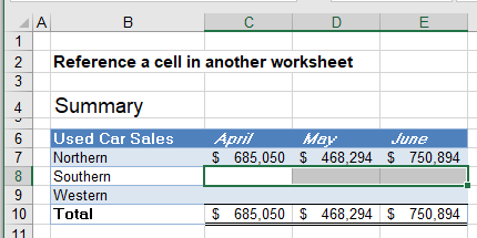
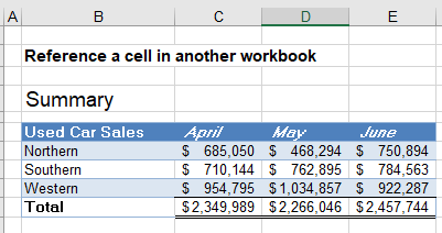
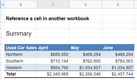
This tutorial will demonstrate how to reference a cell in another sheet in Excel and Google Sheets
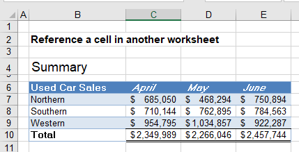
Reference to another Sheet – Create a Formula
In a workbook with multiple worksheets, we can create a formula that will reference a cell in a different worksheet from the one you are working in.
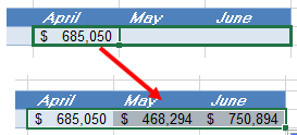
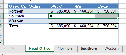
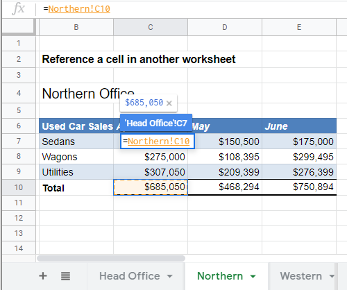
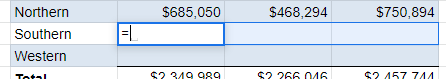
Select the cell where the formula should go ex: C7
Press the equal sign, and then click on the sheet you wish to reference.
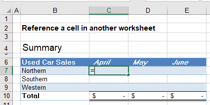
Click on the cell that holds the value you require.
Press Enter or click on the tick in the formula bar.
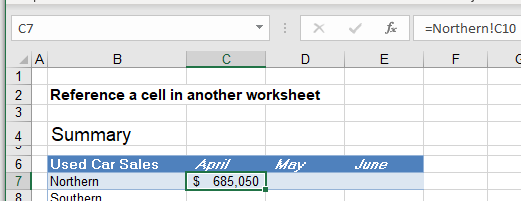
Your formula will now appear with the correct amount in cell C7.
The sheet name will always have an exclamation mark at the end. This is followed by the cell address.
Sheet_name!Cell_address
For example:
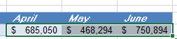
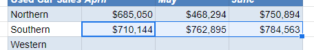
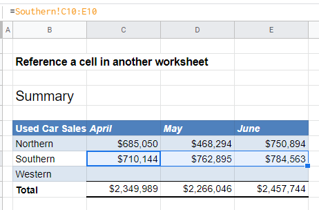
=Northern!C10If your sheet name contains any spaces, then the reference to the sheet will appear in single quotes.
For example:
='Northern Office'!C10Should the value change in the source sheet, then the value of this cell will also change.
You can now drag that formula across to cells D7 and E7 to reference the values in the corresponding cells in the source worksheet.
Reference to Another Sheet – the INDIRECT Function
Instead of typing in the name of the sheet, you can use the INDIRECT Function to get the name of the sheet from a cell that contains the sheets name.
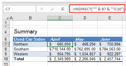
When you reference another sheet in Excel, you usually type the sheet’s name, and then an exclamation mark followed by the cell reference. Since sheet names often contain spaces, we often enclose the name of the sheet in single quotes.
In the formula above therefore, we have used the INDIRECT Function to refer to the name of the sheet in cell B7 ex: “Northern”.
The entire formula above would therefore be
=INDIRECT("'" & Northern & "!C10")where we have replaced the sheet name “Northern” with cell B7.
We can then copy that formula down to C8 and C9 – and the sheet name “Northern” will be replaced with “Southern” and “Western” as the formula is copied down.
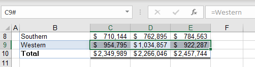
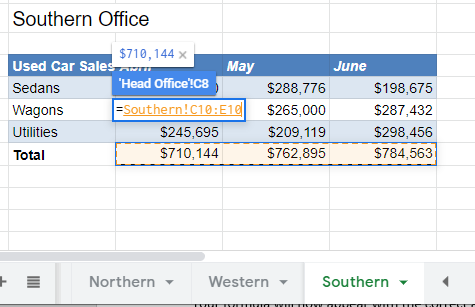
Reference to another Sheet – an Array Formula
To reference to another sheet using an Array formula, select the cells in the Target worksheet first.
For example:
Select C8:E8
Press the equal sign, and then click on the worksheet that contains the Source data.
Highlight the relevant source data cells.
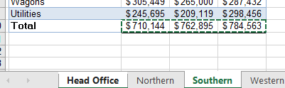
Press Enter to enter the formula into the Target worksheet.
You will notice that the cells contain a range (C10:E10) but that each relevant column will only show the value from the corresponding column in the source workbook.
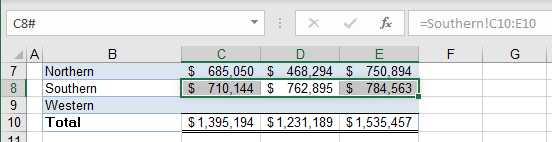
Reference to a Range Name
The array formula is useful when you are referencing to a range name that contains a range of cells and not just a single cell.
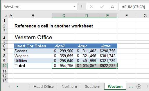
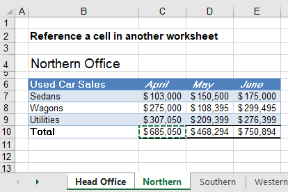
In the above example, the total values of the Western office in row 10 is called Western.
Click in the Head Office sheet, highlight the cells required and press the equal sign on the keyboard.
Type the range name that you have created ex: Western.
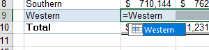
Press Enter.
An array formula will be created.
Reference to another Workbook
You can also link workbooks together by means of referencing to a cell in another workbook.
Have both workbooks open in Excel. You can use the view menu to see them both on the screen if you wish.
Click in the cell you wish to put the source data in ex: C12
Press the equal key on the keyboard and click on the Source cell in the different Workbook.
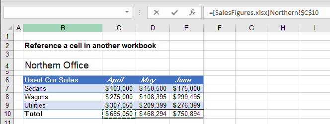
Press Enter.
The formula that is entered into the original sheet will have a reference to the external file, as well as a reference to the sheet name in the external file.
The name of the workbook will be put into square brackets, while the sheet name will always have an exclamation mark at the end. This is followed by the cell address.
[Workbook_name]Sheet_name!Cell_address
For example:
=[SalesFigures.xlsx]Northern!$C$10You will notice that the cell reference has been made an absolute. This means that you CANNOT drag it across to columns D and E unless you remove the absolute.
Click in the cell, and then click in the formula bar and click on the cell address of the formula bar.
Press F4 until the absolute is removed.
![]()
Alternatively, you can delete the $ signs from around the absolute.
Drag the formula across to columns D and E.
Reference to another Sheet in Google Docs
Linking worksheets with formulas works the same way in Google Docs as it does in Excel.
Click in the cell you wish to put the formula into, and then click on the Source cell where your value is stored.
Press Enter.
Your formula will now appear with the correct amount in cell C7.
The sheet name will always have an exclamation mark at the end. This is followed by the cell address.
Sheet_name!Cell_address
For example:
=Northern!C10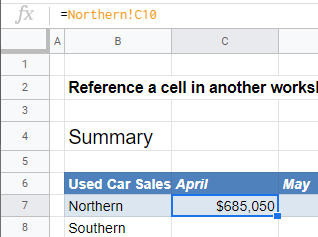
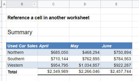
Drag the formula across to populate columns D and E, and then repeat the process for all the sheets.
Reference to another Sheet using an Array Formula in Excel
The array formula will also work in the same way.
Highlight the range you wish to put the target information in and press the equal sign on the keyboard.
Click on the Source sheet and highlight the cells you require.
Press Shift+Enter.
The formula will appear as a range but that each relevant column will only show the value from the corresponding column in the source workbook.
Reference to another Workbook in Google Docs
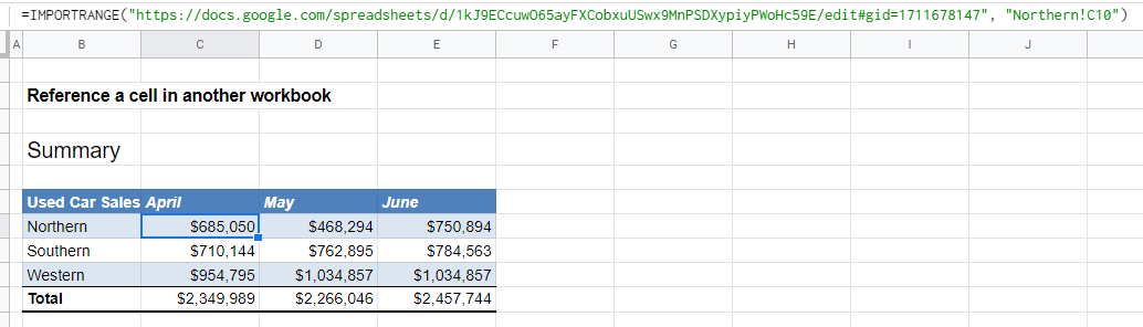
If you want to link Google Sheets files together, you need to use a function called IMPORTRANGE
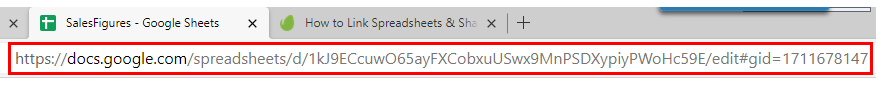
Open the Source Google sheet file in order to copy the URL address of the file.
For example
Return to the sheet where you wish to input the formula and click in the relevant cell.
Press the equal sign on the keyboard and type in the function name ex: IMPORTRANGE, followed by a bracket and inverted commas.
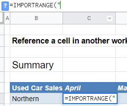
Paste the URL copied from the source Google sheet into the formula.
Close the inverted commas
For example:
=IMPORTRANGE("https://docs.google.com/spreadsheets/d/1kJ9ECcuwO65ayFXCobxuUSwx9MnPSDXypiyPWoHc59E/edit#gid=1711678147"Add another comma and then also in inverted commas, type in the cell reference required
For example
“Northern!C10”
Your complete formula will look like the example below
=IMPORTRANGE("https://docs.google.com/spreadsheets/d/1kJ9ECcuwO65ayFXCobxuUSwx9MnPSDXypiyPWoHc59E/edit#gid=1711678147", "Northern!C10")When you link Google sheets for the first time, this message could appear.
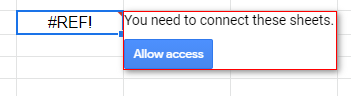
Click Allow access.
Repeat the process for any other cells that need to be linked eg D10 and E10.
TIP: Drag the formula across to the required cells and change the cells address in the formula bar!
In Excel, copying data from one worksheet to another is an easy task, but there is not any link between the two. But we can create a link between two worksheets or workbooks to automatically update data in another sheet if it changes in the first worksheet. This article explains how this is done.
Automatically data in another sheet in Excel
We can link worksheets and update data automatically. A link is a dynamic formula that pulls data from a cell of one worksheet and automatically updates that data to another worksheet. These linking worksheets can be in the same workbook or in another workbook.
One worksheet is called the source worksheet, from where this link pulls the data automatically, and the other worksheet is called the destination worksheet that contains that link formula and where data is updated automatically.
Remember one thing that formatting of cells of source worksheet and destination worksheet should be the same otherwise the result could be viewed differently and can lead to confusion.
Two methods of linking data in different worksheets
We can link these two worksheets using two different methods.
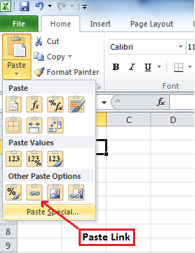
- Copy and Paste Link
- From source worksheet, select the cell that contains data or that you want to link to another worksheet, and copy it by pressing the Copy button from the Home tab or press CTRL+C.
- Go to the destination worksheet and click the cell where you want to link the cell from the source worksheet. On the Home tab, click on the drop-down arrow button of Paste, and select Paste Link from “Other Paste Options.” Or right-click in the cell on the destination worksheet and choose Paste Link from Paste Options.
- Save the work or return to the source workbook and press ESC button on the keyboard to remove the border around the copied cell and save the work.

- Enter formula manually
- In the destination worksheet, click on the cell that will contain link formula and enter an equal sign (=)
- Go to the source sheet and click on the cell that contains data and press Enter on the keyboard. Save your work.
Using these two methods, we can link a worksheet and update data automatically depending upon your requirements. In this article, we will discuss some examples using the following cases.
Update cell on one worksheet based on a cell on another sheet
Suppose we have a value of 200 in cell A1 on Sheet1 and want to update cell A1 on Sheet2 using the linking formula. We can do that by using the same two methods we’ve covered.
Using Copy and Paste Link method
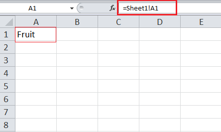
Copy the cell value of 200 from cell A1 on Sheet1.

Go to Sheet2, click in cell A1 and click on the drop-down arrow of Paste button on the Home tab and select Paste Link button. It will generate a link by automatically entering the formula =Sheet1!A1.

Or right-click in the cell on the destination worksheet, Sheet2, and choose Paste Link from Paste Options: It will generate linking formula automatically.

Entering formula manually
We can enter the linking formula manually in cell A1 on the destination worksheet Sheet2 to update data by pulling it from cell A1 of Sheet1.
In cell A1 on Sheet2, manually enter an equal sign (=) and go to Sheet1 and click on cell A1 and press ENTER key on your keyboard. The following linking formula will be updated in destination sheet that will link cell A1 of both sheets.
=Sheet1!A1
Update cell on one sheet only if the first sheet meets a condition
By entering the linking formula manually, we can update data in cell A1 of Sheet2 based on a condition if the cell value of A1 on Sheet1 is greater than 200. We can do that by entering this logical condition in an IF function. If cell A1 on Sheet1 meets this condition then IF function returns the value in cell A1 on Sheet2 otherwise it will return blank cell.
Here is the formula to link the cells of both sheets based on this condition. We will enter this formula manually in cell A1 of Sheet2
=IF(Sheet1!A1>200,Sheet1!A1,"")

Update cell on one sheet from another sheet with a drop-down list
Suppose we have a drop-down list in cell A1 of Sheet1 and we can update cell A1 on Sheet2 by entering link formula in cell A1 on Sheet2.

In cell A1 on Sheet2, we will manually enter this linking formula to update data automatically based on the cell value selected from the drop-down list.
=Sheet1!A1
Linking data in a real data set is more complex and depends on your situation. You might need to use techniques other than those listed above. If you are in a rush and want your problem answered by an Excel expert, try our service. The experts are available to help you 24/7. The first question is free.
A table in Excel is a complex array with set of parameters. It can consist of values, text cells, formulas and be formatted in various ways (cells can have a certain alignment, color, text direction, special notes, etc.).
When you copy a table, sometimes you do not have to transfer all of its elements, but only some of its. Consider how this can be done.
The past special
It is very convenient to carry out the transfer of the data in the table using the past special. It allows you to select only those parameters that we need when copying. Let’s consider an example.
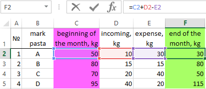
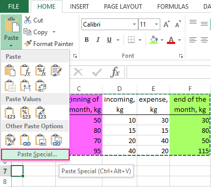
We have the table with the indicators for the presence of macaroni of certain brands in the warehouse of the store. It is clearly visible, how many kilograms were at the beginning of the month, how much of them were bought and sold, and also the balance at the end of the month. Two important columns are highlighted in different colors. The balance at the end of the month is calculated by the elementary formula.
We will try to use the PAST SPECIAL command and copy all the data.
First we select the existing table, right click the menu and click on COPY.
In the free cell, we call the menu again with the right button and press the PAST SPECIAL.
If we leave everything as is by default and just click OK, the table will be inserted completely, with all its parameters.
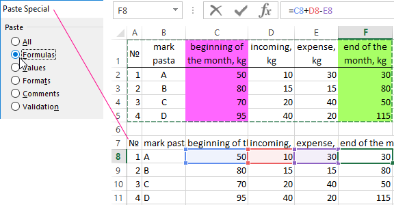
Let’s try to experiment. In the PAST SPECIAL we choose another item, for example, FORMULAS. We have already received an unformatted table, but with working formulas.
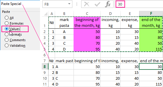
Now we will insert not the formulas, but only the VALUES of the results of calculations.
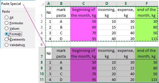
That a new table with values to get the appearance similar to the sample, you need to select it and insert the FORMATS using a special insert.
Now let’s try to choose the item WITHOUT FRAME. We got the full table, but only without the allocated borders.
The wholesome advice! To migrate the format along with the size of the columns, you need to select not the range of the source table, but the entire columns (in this case, the A: F range) before the copying.
Similarly, you can experiment with each item of the PAST SPECIAL to see clearly how it works.
Transfer of data to another sheet
Transferring data to other worksheets in the Excel workbook allows you to link multiple tables. This is convenient because when you replace a value on one sheet, the values change on all the others. When creating annual reports, this is an indispensable thing.
Consider how this works. For a start we rename Excel sheets in months. Then, with the helping of the PAST SPECIAL that we already know, we move the table to February and remove the values from the three columns:
- At the beginning of the month.
- The incoming.
- The expense.
The column «At the end of the month» is given by the formula, so when you delete values from the previous columns, it is automatically reset to zero.
We will transfer to the data on the remainder of macaroni of each brand from January to February. This is done in a couple of clicks.
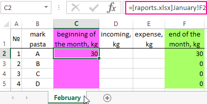
- On the FEBRUARY sheet we place the cursor in the cell, indicating the amount of macaroni of grade A at the beginning of the month. You can see the picture above — this will be cell D3.
- We put in this cell to the sign EQUAL.
- Go to the JANUARY sheet and click on the cell showing the amount of macaroni of grade A at the end of the month (in this case it is cell F2).
We get the following: in the cell C2 the formula was formed, which sends us to the cell F2 of the JANUARY sheet. Stretch the formula down to know the amount of macaroni of each brand at the beginning of February.
Similarly, you can transfer the data to all months and get to the visual annual report.
Data transfer to another file
Similarly, you can transfer data from one file to another one. This book in our example is called EXCEL. Create another one and name it EXAMPLE.
Note. You can create new Excel files even in different folders. The program will automatically search for the specified book, regardless of which folder and on what drive of the computer it is located.
We copy in the book EXAMPLE to the table using the same PAST SPECIAL and again delete the values from the three columns. We will perform the same actions as in the previous paragraph, but we will not go to another sheet, but to another book only.
We have received to the new formula, which shows that the cell refers to the book EXCEL. And we see that the cell =[raports.xlsx]January!F2 looks like =[raports.xlsx]January!$F$2, i. e. it is fixed. And if we want to stretch to the formula in other brands of macaroni, first you need to remove the dollar badges for removing to the commit.
Now you know how to correctly transfer data from tables within one sheet, from one sheet to another, and from one file to another one.
When working with excel sheets, you may have similar data that you are working with and which are in different excel sheets. Such data can be pulled from one of the sheets to another. This will save time in writing data in the columns or rows again.
To pull data from one excel sheet to another is the process of taking the data, be it in a column or a row, to another excel sheet. Once we pull values from another sheet, which is commonly done, we can save on time taken which we would otherwise keep in inserting the values in columns or rows.
Errors are minimized because while inserting the data all over again; you may omit some values, which will cause issues in the data set.
We have several procedures to follow to pull data from other sheets; the steps involved include the ones below;
Using Enter and Save
First, open a new excel sheet; in sheet 1, insert data as in the case below.

Leave the column with the estate as the header empty.
In sheet 2, enter the data as follows and save the excel sheet as «sheet2«

Using VLOOKUP Function
Having our sheets set with data values, we will now try and see if we can pull the values from sheet 2 to sheet 1. We have a function that we are going to use; the VLOOKUP function. This function will help us pull data values from sheet 2 to sheet 1. You can also pull data values from any other sheet you wish.
The formula that we will write on the formula bar of sheet 1 will be; = VLOOKUP (B3, ‘Sheet 2’! $B$3: $C$6, 2, 0). This formula on column B values will keep changing because B3 is only the first cell.

The formula will be able to pull the values of column C from sheet 2 upon clicking on the enter button, as in the case below.

The values will automatically be displayed in column C with the header Estate in both sheet 1 and sheet 1.
Using Advanced Filter in Excel
The Advanced Filter is among the easiest ways to use if you want to pull data from another sheet in Excel. For example, you can use it to pull data of customers and their payment details from one sheet and record it in the new worksheet. In this case, you can follow these simple steps:
1. Open the second spreadsheet and click on the Data button.

2. Select the Advanced option from the Sort and Filter commands.

3. A new dialogue box will show up. Select the Copy to another location option under the Action menu.

4. Next, fill in the List range box from the original worksheet. You can also click on the up-facing arrow to select the range directly.
5. Click on the Criteria range and select the data based on the criteria you want.
6. Finish by selecting the cell where you want the extracted data to appear and click the OK button.

If you wanted to pull data of customers who paid using their cards, you get your result showing only those who paid with cards in your preferred range of cells.
Using Combined INDEX And MATCH Functions
You can also combine INDEX and MATCH functions to pull data from one sheet to another based on your preferred criteria. The combination is among the powerful Excel hacks; hence, you can use it to extract customers’ payment details such as amount or payment mode. When using the combination, the MATCH function locates the matching value from the array of another sheet, while the INDEX function returns that value from the list. To pull data on customers’ amounts, you can follow these steps:
1. On a new sheet, select the cell you want to pull from the source sheet. For example, you can select cell D5, which has the customers’ value.
2. Write the following formula in the cell:
=INDEX(‘INDEX & MATCH Functions’!B5:E5,MATCH($B$5,’INDEX & MATCH Functions’!$B$4:$E$4,0))

3. Press the Enter key, and you will see the extracted amount in the new cell.
4. You can now use the cursor or Fill Handle to drag the formula down the column. This will automatically pull data from the source sheet to the new column.

Using the HLOOKUP Function
The HLOOKUP is a unique function to look up data horizontally and bring back the value. For instance, you can use it to pull out customers’ payment history into another worksheet through the following steps:
1. On the new sheet, select the cell with the dataset you want to pull out. For example, you can select cell E5.
2. Write the following formula in the cell and press the Enter button.
=HLOOKUP($B$5,’HLOOKUP Function’!$B$4:$E$8,Sheet4!D5+1,0)

3. You can now use the cursor or Fill Handle to drag the formula down the cells.
4. The function will pull out all the customers’ payment history from the source sheet and return the data to the new sheet.

Using Cell References
Of all the methods, using relevant cell references is the simplest way to pull data from one Excel sheet to another. Here, you can use these steps:
1. Select the cell where you want the extracted data to appear.

2. Type the equal sign (=) followed by the name of the sheet you want to pull data from. Enclose the sheet name in single quote marks if the name of the sheet is more than one word. Type the ‘!’ sign followed by the cell reference of the cell you to pull data from.

3. Press the Enter button, and the data from your source sheet will appear in the new cell.
4. You can now drag the Fill Handle (+) icon down the column to pull data from other remaining cells.
