Формула isblank if excel - Word и Excel - помощь в работе с программами

Excel for Microsoft 365 Excel for Microsoft 365 for Mac Excel 2021 Excel 2021 for Mac Excel 2019 Excel 2019 for Mac Excel 2016 Excel 2016 for Mac Excel 2013 Excel 2010 Excel 2007 Excel for Mac 2011 More…Less

Sometimes you need to check if a cell is blank, generally because you might not want a formula to display a result without input.

In this case we’re using IF with the ISBLANK function:

=IF(ISBLANK(D2),»Blank»,»Not Blank»)

Which says IF(D2 is blank, then return «Blank», otherwise return «Not Blank»). You could just as easily use your own formula for the «Not Blank» condition as well. In the next example we’re using «» instead of ISBLANK. The «» essentially means «nothing».

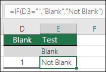
=IF(D3=»»,»Blank»,»Not Blank»)

This formula says IF(D3 is nothing, then return «Blank», otherwise «Not Blank»). Here is an example of a very common method of using «» to prevent a formula from calculating if a dependent cell is blank:

=IF(D3=»»,»»,YourFormula())

IF(D3 is nothing, then return nothing, otherwise calculate your formula).

Need more help?

Want more options?

Explore subscription benefits, browse training courses, learn how to secure your device, and more.

Communities help you ask and answer questions, give feedback, and hear from experts with rich knowledge.

Источник

The ISBLANK function returns TRUE when a cell is empty, and FALSE when a cell is not empty. For example, if A1 contains «apple», ISBLANK(A1) returns FALSE. Use the ISBLANK function to test if a cell is empty or not. ISBLANK function takes one argument, value, which is a cell reference like A1.

The word «blank» is somewhat misleading in Excel, because a cell that contains only space will look blank but not be empty. In general, it is best to think of ISBLANK to mean «is empty» since it will return FALSE when a cell looks blank but is not empty.

Examples

If cell A1 contains nothing at all, the ISBLANK function will return TRUE:

=ISBLANK(A1) // returns TRUE

If cell A1 contains any value, or any formula, the ISBLANK function will return FALSE:

=ISBLANK(A1) // returns false

Is not blank

To test if a cell is not blank, nest ISBLANK inside the NOT function like this:

=NOT(ISBLANK(A1)) // test not blank

The above formula will return TRUE when a cell is not empty, and FALSE when a cell is empty.

Empty string syntax

Many formulas will use an abbreviated syntax to test for empty cells, instead of the ISBLANK function. This syntax uses an empty string («») with Excel’s math operators «=» or «<>». For example, to test if A1 is empty, you can use:

=A1="" // TRUE if A1 is empty

To test if A1 is not empty:

=A1<>"" // TRUE if A1 is not empty

This syntax can be used interchangeably with ISBLANK. For example, inside the IF function:

=IF(ISBLANK(A1),result1,result2) // if A1 is empty

is equivalent to:

=IF(A1="",result1,result2) // if A1 is empty

Likewise, the formula:

=IF(NOT(ISBLANK(A1)),result1,result2)

is the same, as:

=IF(A1<>"",result1,result2)

Both will return result1 when A1 is not empty, and result2 when A1 is empty.

Empty strings

If a cell contains any formula, the ISBLANK function and the alternatives above will return FALSE, even if the formula returns an empty string («»). This can cause problems when the goal is to count or process blank cells that include empty strings.

One workaround is to use the LEN function to test for a length of zero. For example, the formula below will return TRUE if A1 is empty or contains a formula that returns an empty string:

=LEN(A1)=0 // TRUE if empty

So, inside the IF function, you can use LEN like this:

=IF(LEN(A1)=0,result1,result2) // if A1 is empty

You can use this same approach to count cells that are not blank.

Источник

Скачать пример рабочей книги

Загрузите образец книги

В этом руководстве показано, как использовать Функция Excel ISBLANK в Excel, чтобы проверить, пуста ли ячейка.

Функциональный тест ISBLANK, если ячейка пуста. Возвращает ИСТИНА или ЛОЖЬ.

Чтобы использовать функцию ISBLANK Excel Worksheet, выберите ячейку и введите:

(Обратите внимание, как появляются входные данные формулы)

Синтаксис и входные данные функции ISBLANK:

ценить — Тестовое значение

Как использовать функцию ISBLANK

Функция ISBLANK проверяет, является ли ячейка полностью пусто или нет. Он возвращает ИСТИНА, если ячейка пуста, в противном случае — ЛОЖЬ.

Если ячейка пуста, то

Часто вам нужно объединить функцию «IS», например ISBLANK, с функцией IF. С помощью функции ЕСЛИ вместо того, чтобы возвращать простое значение ИСТИНА или ЛОЖЬ, вы можете выводить определенный текст или выполнять определенные действия, если ячейка пуста или нет.

1	= ЕСЛИ (ISBLANK (C2); «»; C2 * D2)

ЕСЛИ ячейка не пуста, то

С помощью функции НЕ вы можете проверить обратное: ячейка не пуста?

1	= ЕСЛИ (НЕ (ПУСТОЙ (C2)); C2 * D2; «»)

Диапазон ISBLANK — СЧИТАТЬПУСТОТЫ

Чтобы проверить диапазон на наличие пустых значений, вы можете использовать функцию ISBLANK вместе с функцией SUMPRODUCT. Однако самый простой способ проверить наличие пустых ячеек — использовать функцию СЧИТАТЬПУСТОТЫ.

Функция СЧИТАТЬПУСТОТЫ подсчитывает количество пустых ячеек в диапазоне.

1	= СЧИТАТЬПУСТОТЫ (A2: C7)

Если СЧИТАТЬПУСТОТЫ> 0, то в диапазоне есть хотя бы одна пустая ячейка. Используйте это вместе с оператором IF, чтобы что-то сделать, если будет обнаружена пустая ячейка.

1	= ЕСЛИ (СЧИТАТЬ ПУСТОЙ (A2: C2)> 0,100 * СУММ (A2: C2); 200 * СУММ (A2: C2))

Функция ISBLANK не работает?

Функция ISBLANK вернет FALSE для ячеек, которые выглядят пустыми, но это не так. Включая:

Строка нулевой длины из внешнего источника данных
пробелы, апострофы, неразрывные пробелы () или другие непечатаемые символы.
Пустая строка («»)

Используя функции ЕСЛИ и ИЛИ, вы можете идентифицировать ячейки с пустыми строками, а также с обычными пустыми ячейками.

1	= ЕСЛИ (ИЛИ (ISBLANK (A2), A2 = «»), «пробел», «не пробел»)

Другой вариант — использовать функцию TRIM для удаления лишних пробелов и функцию LEN для подсчета количества символов.

1	= ЕСЛИ (ИЛИ (A2 = «», LEN (TRIM (A2)) = 0), «пусто», «не пусто»)

Другие логические функции

Таблицы Excel / Google содержат множество других логических функций для выполнения других логических тестов. Вот список:

IF / IS функции
если ошибка
ошибка
Исна
iserr
пусто
это число
istext
нетекст
isformula
логичен
isref
даже
isodd

ISBLANK в Google Таблицах

Функция ISBLANK работает в Google Таблицах точно так же, как и в Excel:

Вы поможете развитию сайта, поделившись страницей с друзьями

Источник

Home / Excel Formulas / IF Cell is Blank (Empty) using IF + ISBLANK

In Excel, if you want to check if a cell is blank or not, you can use a combination formula of IF and ISBLANK. These two formulas work in a way where ISBLANK checks for the cell value and then IF returns a meaningful full message (specified by you) in return.

In the following example, you have a list of numbers where you have a few cells blank.

Formula to Check IF a Cell is Blank or Not (Empty)

First, in cell B1, enter IF in the cell.
Now, in the first argument, enter the ISBLANK and refer to cell A1 and enter the closing parentheses.
Next, in the second argument, use the “Blank” value.
After that, in the third argument, use “Non-Blank”.
In the end, close the function, hit enter, and drag the formula up to the last value that you have in the list.

As you can see, we have the value “Blank” for the cell where the cell is empty in column A.

=IF(ISBLANK(A1),"Blank","Non-Blank")

Now let’s understand this formula. In the first part where we have the ISBLANK which checks if the cells are blank or not.

And, after that, if the value returned by the ISBLANK is TRUE, IF will return “Blank”, and if the value returned by the ISBLANK is FALSE IF will return “Non_Blank”.

Alternate Formula

You can also use an alternate formula where you just need to use the IF function. Now in the function, you just need to specify the cell where you want to test the condition and then use an equal operator with the blank value to create a condition to test.

And you just need to specify two values that you want to get the condition TRUE or FALSE.

Download Sample File

Ready

And, if you want to Get Smarter than Your Colleagues check out these FREE COURSES to Learn Excel, Excel Skills, and Excel Tips and Tricks.

Источник

Функция ЕСЛИ в Excel — это отличный инструмент для проверки условий на ИСТИНУ или ЛОЖЬ. Если значения ваших расчетов равны заданным параметрам функции как ИСТИНА, то она возвращает одно значение, если ЛОЖЬ, то другое.

Содержание

Что возвращает функция
Синтаксис
Аргументы функции
Дополнительная информация
Функция Если в Excel примеры с несколькими условиями
Пример 1. Проверяем простое числовое условие с помощью функции IF (ЕСЛИ)
Пример 2. Использование вложенной функции IF (ЕСЛИ) для проверки условия выражения
Пример 3. Вычисляем сумму комиссии с продаж с помощью функции IF (ЕСЛИ) в Excel
Пример 4. Используем логические операторы (AND/OR) (И/ИЛИ) в функции IF (ЕСЛИ) в Excel
Пример 5. Преобразуем ошибки в значения “0” с помощью функции IF (ЕСЛИ)

Что возвращает функция

Заданное вами значение при выполнении двух условий ИСТИНА или ЛОЖЬ.

Синтаксис

=IF(logical_test, [value_if_true], [value_if_false]) — английская версия

=ЕСЛИ(лог_выражение; [значение_если_истина]; [значение_если_ложь]) — русская версия

Аргументы функции

logical_test (лог_выражение) — это условие, которое вы хотите протестировать. Этот аргумент функции должен быть логичным и определяемым как ЛОЖЬ или ИСТИНА. Аргументом может быть как статичное значение, так и результат функции, вычисления;
[value_if_true] ([значение_если_истина]) — (не обязательно) — это то значение, которое возвращает функция. Оно будет отображено в случае, если значение которое вы тестируете соответствует условию ИСТИНА;
[value_if_false] ([значение_если_ложь]) — (не обязательно) — это то значение, которое возвращает функция. Оно будет отображено в случае, если условие, которое вы тестируете соответствует условию ЛОЖЬ.

Дополнительная информация

В функции ЕСЛИ может быть протестировано 64 условий за один раз;
Если какой-либо из аргументов функции является массивом — оценивается каждый элемент массива;
Если вы не укажете условие аргумента FALSE (ЛОЖЬ) value_if_false (значение_если_ложь) в функции, т.е. после аргумента value_if_true (значение_если_истина) есть только запятая (точка с запятой), функция вернет значение “0”, если результат вычисления функции будет равен FALSE (ЛОЖЬ).
На примере ниже, формула =IF(A1> 20,”Разрешить”) или =ЕСЛИ(A1>20;»Разрешить») , где value_if_false (значение_если_ложь) не указано, однако аргумент value_if_true (значение_если_истина) по-прежнему следует через запятую. Функция вернет “0” всякий раз, когда проверяемое условие не будет соответствовать условиям TRUE (ИСТИНА).

|
Если вы не укажете условие аргумента TRUE(ИСТИНА) (value_if_true (значение_если_истина)) в функции, т.е. условие указано только для аргумента value_if_false (значение_если_ложь), то формула вернет значение “0”, если результат вычисления функции будет равен TRUE (ИСТИНА);
На примере ниже формула равна =IF (A1>20;«Отказать») или =ЕСЛИ(A1>20;»Отказать»), где аргумент value_if_true (значение_если_истина) не указан, формула будет возвращать “0” всякий раз, когда условие соответствует TRUE (ИСТИНА).

Функция Если в Excel примеры с несколькими условиями

Пример 1. Проверяем простое числовое условие с помощью функции IF (ЕСЛИ)

При использовании функции ЕСЛИ в Excel, вы можете использовать различные операторы для проверки состояния. Вот список операторов, которые вы можете использовать:

Ниже приведен простой пример использования функции при расчете оценок студентов. Если сумма баллов больше или равна «35», то формула возвращает “Сдал”, иначе возвращается “Не сдал”.

Пример 2. Использование вложенной функции IF (ЕСЛИ) для проверки условия выражения

Функция может принимать до 64 условий одновременно. Несмотря на то, что создавать длинные вложенные функции нецелесообразно, то в редких случаях вы можете создать формулу, которая множество условий последовательно.

В приведенном ниже примере мы проверяем два условия.

Первое условие проверяет, сумму баллов не меньше ли она чем 35 баллов. Если это ИСТИНА, то функция вернет “Не сдал”;
В случае, если первое условие — ЛОЖЬ, и сумма баллов больше 35, то функция проверяет второе условие. В случае если сумма баллов больше или равна 75. Если это правда, то функция возвращает значение “Отлично”, в других случаях функция возвращает “Сдал”.

Пример 3. Вычисляем сумму комиссии с продаж с помощью функции IF (ЕСЛИ) в Excel

Функция позволяет выполнять вычисления с числами. Хороший пример использования — расчет комиссии продаж для торгового представителя.

В приведенном ниже примере, торговый представитель по продажам:

не получает комиссионных, если объем продаж меньше 50 тыс;
получает комиссию в размере 2%, если продажи между 50-100 тыс
получает 4% комиссионных, если объем продаж превышает 100 тыс.

Рассчитать размер комиссионных для торгового агента можно по следующей формуле:

=IF(B2<50,0,IF(B2<100,B2*2%,B2*4%)) — английская версия

=ЕСЛИ(B2<50;0;ЕСЛИ(B2<100;B2*2%;B2*4%)) — русская версия

В формуле, использованной в примере выше, вычисление суммы комиссионных выполняется в самой функции ЕСЛИ. Если объем продаж находится между 50-100K, то формула возвращает B2 * 2%, что составляет 2% комиссии в зависимости от объема продажи.

Больше лайфхаков в нашем Telegram Подписаться

Пример 4. Используем логические операторы (AND/OR) (И/ИЛИ) в функции IF (ЕСЛИ) в Excel

Вы можете использовать логические операторы (AND/OR) (И/ИЛИ) внутри функции для одновременного тестирования нескольких условий.

Например, предположим, что вы должны выбрать студентов для стипендий, основываясь на оценках и посещаемости. В приведенном ниже примере учащийся имеет право на участие только в том случае, если он набрал более 80 баллов и имеет посещаемость более 80%.

Вы можете использовать функцию AND (И) вместе с функцией IF (ЕСЛИ), чтобы сначала проверить, выполняются ли оба эти условия или нет. Если условия соблюдены, функция возвращает “Имеет право”, в противном случае она возвращает “Не имеет право”.

Формула для этого расчета:

=IF(AND(B2>80,C2>80%),”Да”,”Нет”) — английская версия

=ЕСЛИ(И(B2>80;C2>80%);»Да»;»Нет») — русская версия

Пример 5. Преобразуем ошибки в значения “0” с помощью функции IF (ЕСЛИ)

С помощью этой функции вы также можете убирать ячейки содержащие ошибки. Вы можете преобразовать значения ошибок в пробелы или нули или любое другое значение.

Формула для преобразования ошибок в ячейках следующая:

=IF(ISERROR(A1),0,A1) — английская версия

=ЕСЛИ(ЕОШИБКА(A1);0;A1) — русская версия

Формула возвращает “0”, в случае если в ячейке есть ошибка, иначе она возвращает значение ячейки.

ПРИМЕЧАНИЕ. Если вы используете Excel 2007 или версии после него, вы также можете использовать функцию IFERROR для этого.

Точно так же вы можете обрабатывать пустые ячейки. В случае пустых ячеек используйте функцию ISBLANK, на примере ниже:

=IF(ISBLANK(A1),0,A1) — английская версия

=ЕСЛИ(ЕПУСТО(A1);0;A1) — русская версия

Источник

В группу функций Е входит девять функций, которые проверяют значение, и, в зависимости от результата, возвращают значение ИСТИНА либо ЛОЖЬ.

Описание функций группы Е

Каждая из функций Е проверяет указанное значение и возвращает в зависимости от результата значение ИСТИНА или ЛОЖЬ. Всего девять функций: ЕПУСТО, ЕОШ, ЕОШИБКА, ЕЛОГИЧ, ЕНД, ЕНЕТЕКСТ, ЕЧИСЛО, ЕССЫЛКА, ЕТЕКСТ.

Например, функция ЕПУСТО возвращает логическое значение ИСТИНА, если проверяемое значение является ссылкой на пустую ячейку; в противном случае возвращается логическое значение ЛОЖЬ. Функции Е используются для получения сведений о значении перед выполнением с ним вычисления или другого действия.

Например, для выполнения другого действия при возникновении ошибки можно использовать функцию ЕОШИБКА в сочетании с функцией ЕСЛИ:

=ЕСЛИ(ЕОШИБКА(A1);"Произошла ошибка.";A1*2)

Эта формула проверяет наличие ошибки в ячейке A1. При возникновении ошибки функция ЕСЛИ возвращает сообщение «Произошла ошибка.» Если ошибки отсутствуют, функция ЕСЛИ вычисляет произведение A1*2.

Синтаксис

=ЕПУСТО(значение)

Аргументы

значение

Обязательный аргумент. Значением этого аргумента может быть пустая ячейка, значение ошибки, логическое значение, текст, число, ссылка на любой из перечисленных объектов или имя такого объекта.

Функция ЕПУСТО возвращает значение ИСТИНА, если аргумент «значение» ссылается на пустую ячейку.

Замечания

Аргументы в функциях Е не преобразуются. Любые числа, заключенные в кавычки, воспринимаются как текст. Например, в большинстве других функций, требующих числового аргумента, текстовое значение «19» преобразуется в число 19. Однако в формуле ЕЧИСЛО(«19») это значение не преобразуется из текста в число, и функция ЕЧИСЛО возвращает значение ЛОЖЬ.
С помощью этих функций удобно проверять результаты вычислений в формулах. Комбинируя эти функции с функцией ЕСЛИ, можно находить ошибки в формулах.

Пример

Источник

Date yes Add (Subtract) Days to a Date Concatenate Dates Convert Date to Number Convert Date to Text Month Name to Number Create Date Range from Dates Day Number of Year Month Name from Date First Day of Month Add (Subtract) Weeks to a Date If Functions with Dates Max Date Number of Days Between Dates Number of Days in a Month Number of Weeks Between Dates Number of Years Between Dates Split Date & Time into Separate Cells Countdown Remaining Days Insert Dates Random Date Generator Using Dynamic Ranges — Year to Date Values Add (Subtract) Years to a Date Date Formula Examples Extract Day from Date Get Day Name from Date Count Days Left in Month / Year Count Workdays Left in Month / Year Get Last Day of Month Last Business Day of Month / Year Number of Work / Business Days in Month Weekday Abbreviations Auto Populate Dates Number of Months Between Dates Quarter from a Date Years of Service Change Date Format Compare Dates Time yes Add (Subtract) Hours to Time Add (Subtract) Minutes to Time Add (Subtract) Seconds to Time Add Up time (Total Time) Time Differences Change Time Format Convert Minutes to Hours Convert Time to Decimal Convert Time to Hours Convert Time to Minutes Convert Time to Seconds Military Time Round Time to Nearest 15 Minutes Overtime Calculator Number of Hours Between Times Convert Seconds to Minutes, Hours, or Time Count Hours Worked Time Differences Time Format — Show Minutes Seconds Text yes Add Commas to Cells Get First Word from Text Capitalize First Letter Clean & Format Phone #s Remove Extra Trailing / Leading Spaces Add Spaces to Cell Assign Number Value to Text Combine Cells with Comma Combine First and Last Names Convert Text String to Date Convert Text to Number Extract Text From Cell Get Last Word Remove Unwated Characters Extract Text Before or After Character How to Split Text String by Space, Comma, & More Remove Special Characters Remove First Characters from Left Substitute Multiple Values Switch First & Last Names w/ Commas Remove Specific Text from a Cell Extract Text Between Characters (Ex. Parenthesis) Add Leading Zeros to a Number Remove Line Breaks from Text Remove all Numbers from Text Reverse Text Remove Non-Numeric Characters Remove Last Character(s) From Right Separate First and Last Names Separate Text & Numbers Round yes Round Formulas Round Price to Nearest Dollar or Cent Round to Nearest 10, 100, or 1000 Round to Nearest 5 or .5 Round Percentages Round to Significant Figures Count yes Count Blank and Non-blank Cells Count Cells Between Two Numbers Count Cells not Equal to Count if Cells are in Range Count Times Word Appears in Cell Count Words in Cell Count Specific Characters in Column Count Total Number of Characters in Column Count Cells that Equal one of two Results Count Cells that do not Contain Count Cells that Contain Specific Text Count Unique Values in Range Countif — Multiple Criteria Count Total Number of Cells in Range Count Cells with Any Text Count Total Cells in a Table Lookup yes Two Dimensional VLOOKUP VLOOKUP Simple Example Vlookup — Multiple Matches Case Sensitive Lookup Case Sensitive VLOOKUP Sum if — VLOOKUP Case Sensitive Lookup Case Sensitive VLOOKUP Find Duplicates w/ VLOOKUP or MATCH INDEX MATCH MATCH Lookup — Return Cell Address (Not Value) Lookup Last Value in Column or Row Reverse VLOOKUP (Right to Left) Risk Score Bucket with VLOOKUP Sum with a VLOOKUP Function VLOOKUP & INDIRECT VLOOKUP Concatenate VLOOKUP Contains (Partial Match) 17 Reasons Why Your XLOOKUP is Not Working Double (Nested) XLOOKUP — Dynamic Columns IFERROR (& IFNA) XLOOKUP Lookup Min / Max Value Nested VLOOKUP Top 11 Alternatives to VLOOKUP (Updated 2022!) VLOOKUP – Dynamic Column Reference VLOOKUP – Fix #N/A Error VLOOKUP – Multiple Sheets at Once VLOOKUP & HLOOKUP Combined VLOOKUP & MATCH Combined VLOOKUP Between Worksheets or Spreadsheets VLOOKUP Duplicate Values VLOOKUP Letter Grades VLOOKUP Return Multiple Columns VLOOKUP Returns 0? Return Blank Instead VLOOKUP w/o #N/A Error XLOOKUP Multiple Sheets at Once XLOOKUP Between Worksheets or Spreadsheets XLOOKUP by Date XLOOKUP Duplicate Values XLOOKUP Multiple Criteria XLOOKUP Return Multiple Columns XLOOKUP Returns 0? Return Blank Instead XLOOKUP Text XLOOKUP with IF XLOOKUP With If Statement Misc. yes Sort Multiple Columns Use Cell Value in Formula Percentage Change Between Numbers Percentage Breakdown Rank Values Add Spaces to Cell CAGR Formula Average Time Decimal Part of Number Integer Part of a Number Compare Items in a List Dealing with NA() Errors Get Worksheet Name Wildcard Characters Hyperlink to Current Folder Compound Interest Formula Percentage Increase Create Random Groups Sort with the Small and Large Functions Non-volatile Function Alternatives Decrease a Number by a Percentage Calculate Percent Variance Profit Margin Calculator Convert Column Number to Letter Get Full Address of Named Range Insert File Name Insert Path Latitute / Longitude Functions Replace Negative Values Reverse List Range Convert State Name to Abbreviation Create Dynamic Hyperlinks Custom Sort List with Formula Data Validation — Custom Formulas Dynamic Sheet Reference (INDIRECT) Reference Cell in Another Sheet or Workbook Get Cell Value by Address Get Worksheet Name Increment Cell Reference List Sheet Names List Skipped Numbers in Sequence Return Address of Max Value in Range Search by Keywords Select Every Other (or Every nth) Row Basics yes Cell Reference Basics — A1, R1C1, 3d, etc. Add Up (Sum) Entire Column or Row Into to Dynamic Array Formulas Conversions yes Convert Time Zones Convert Celsius to Fahrenheit Convert Pounds to Kilograms Convert Time to Unix Time Convert Feet to Meters Convert Centimeters to Inches Convert Kilometers to Miles Convert Inches to Feet Convert Date to Julian Format Convert Column Letter to Number Tests yes Test if a Range Contains any Text Test if any Cell in Range is Number Test if a Cell Contains a Specific Value Test if Cell Contains Any Number Test if Cell Contains Specific Number Test if Cell is Number or Text If yes Percentile If Subtotal If Sumproduct If Large If and Small If Median If Concatentate If Max If Rank If TEXTJOIN If Sum yes Sum if — Begins With / Ends With Sum if — Month or Year to Date Sum if — By Year Sum if — Blank / Non-Blank Sum if — Horizontal Sum Count / Sum If — Cell Color INDIRECT Sum Sum If — Across Multiple Sheets Sum If — By Month Sum If — Cells Not Equal To Sum If — Not Blank Sum if — Between Values Sum If — Week Number Sum Text Sum if — By Category or Group Sum if — Cell Contains Specific Text (Wildcards) Sum if — Date Rnage Sum if — Dates Equal Sum if — Day of Week Sum if — Greater Than Sum if — Less Than Average yes Average Non-Zero Values Average If — Not Blank Average — Ignore 0 Average — Ignore Errors Math yes Multiplication Table Cube Roots nth Roots Square Numbers Square Roots Calculations yes Calculate a Ratio Calculate Age KILLLLLLL Calculate Loan Payments GPA Formula Calculate VAT Tax How to Grade Formulas Find yes Find a Number in a Column / Workbook Find Most Frequent Numbers Find Smallest n Values Find nth Occurance of Character in Text Find and Extract Number from String Find Earliest or Latest Date Based on Criteria Find First Cell with Any Value Find Last Row Find Last Row with Data Find Missing Values Find Largest n Values Most Frequent Number Conditional Formatting yes Conditional Format — Dates & Times Conditional Format — Highlight Blank Cells New Functions XLOOKUP Replaces VLOOKUP, HLOOKUP, and INDEX / MATCH Logical yes AND Checks whether all conditions are met. TRUE/FALSE IF If condition is met, do something, if not, do something else. IFERROR If result is an error then do something else. NOT Changes TRUE to FALSE and FALSE to TRUE. OR Checks whether any conditions are met. TRUE/FALSE XOR Checks whether one and only one condition is met. TRUE/FALSE Lookup & Reference yes FALSE The logical value: FALSE. TRUE The logical value: TRUE. ADDRESS Returns a cell address as text. AREAS Returns the number of areas in a reference. CHOOSE Chooses a value from a list based on it’s position number. COLUMN Returns the column number of a cell reference. COLUMNS Returns the number of columns in an array. HLOOKUP Lookup a value in the first row and return a value. HYPERLINK Creates a clickable link. INDEX Returns a value based on it’s column and row numbers. INDIRECT Creates a cell reference from text. LOOKUP Looks up values either horizontally or vertically. MATCH Searches for a value in a list and returns its position. OFFSET Creates a reference offset from a starting point. ROW Returns the row number of a cell reference. ROWS Returns the number of rows in an array. TRANSPOSE Flips the oriention of a range of cells. VLOOKUP Lookup a value in the first column and return a value. Date & Time yes DATE Returns a date from year, month, and day. DATEDIF Number of days, months or years between two dates. DATEVALUE Converts a date stored as text into a valid date DAY Returns the day as a number (1-31). DAYS Returns the number of days between two dates. DAYS360 Returns days between 2 dates in a 360 day year. EDATE Returns a date, n months away from a start date. EOMONTH Returns the last day of the month, n months away date. HOUR Returns the hour as a number (0-23). MINUTE Returns the minute as a number (0-59). MONTH Returns the month as a number (1-12). NETWORKDAYS Number of working days between 2 dates. NETWORKDAYS.INTL Working days between 2 dates, custom weekends. NOW Returns the current date and time. SECOND Returns the second as a number (0-59) TIME Returns the time from a hour, minute, and second. TIMEVALUE Converts a time stored as text into a valid time. TODAY Returns the current date. WEEKDAY Returns the day of the week as a number (1-7). WEEKNUM Returns the week number in a year (1-52). WORKDAY The date n working days from a date. WORKDAY.INTL The date n working days from a date, custom weekends. YEAR Returns the year. YEARFRAC Returns the fraction of a year between 2 dates. Engineering yes CONVERT Convert number from one unit to another. Financial yes FV Calculates the future value. PV Calculates the present value. NPER Calculates the total number of payment periods. PMT Calculates the payment amount. RATE Calculates the interest Rate. NPV Calculates the net present value. IRR The internal rate of return for a set of periodic CFs. XIRR The internal rate of return for a set of non-periodic CFs. PRICE Calculates the price of a bond. YIELD Calculates the bond yield. INTRATE The interest rate of a fully invested security. Information yes CELL Returns information about a cell. ERROR.TYPE Returns a value representing the cell error. ISBLANK Test if cell is blank. TRUE/FALSE ISERR Test if cell value is an error, ignores #N/A. TRUE/FALSE ISERROR Test if cell value is an error. TRUE/FALSE ISEVEN Test if cell value is even. TRUE/FALSE ISFORMULA Test if cell is a formula. TRUE/FALSE ISLOGICAL Test if cell is logical (TRUE or FALSE). TRUE/FALSE ISNA Test if cell value is #N/A. TRUE/FALSE ISNONTEXT Test if cell is not text (blank cells are not text). TRUE/FALSE ISNUMBER Test if cell is a number. TRUE/FALSE ISODD Test if cell value is odd. TRUE/FALSE ISREF Test if cell value is a reference. TRUE/FALSE ISTEXT Test if cell is text. TRUE/FALSE N Converts a value to a number. NA Returns the error: #N/A. TYPE Returns the type of value in a cell. Math yes ABS Calculates the absolute value of a number. AGGREGATE Define and perform calculations for a database or a list. CEILING Rounds a number up, to the nearest specified multiple. COS Returns the cosine of an angle. DEGREES Converts radians to degrees. DSUM Sums database records that meet certain criteria. EVEN Rounds to the nearest even integer. EXP Calculates the exponential value for a given number. FACT Returns the factorial. FLOOR Rounds a number down, to the nearest specified multiple. GCD Returns the greatest common divisor. INT Rounds a number down to the nearest integer. LCM Returns the least common multiple. LN Returns the natural logarithm of a number. LOG Returns the logarithm of a number to a specified base. LOG10 Returns the base-10 logarithm of a number. MOD Returns the remainder after dividing. MROUND Rounds a number to a specified multiple. ODD Rounds to the nearest odd integer. PI The value of PI. POWER Calculates a number raised to a power. PRODUCT Multiplies an array of numbers. QUOTIENT Returns the integer result of division. RADIANS Converts an angle into radians. RAND Calculates a random number between 0 and 1. RANDBETWEEN Calculates a random number between two numbers. ROUND Rounds a number to a specified number of digits. ROUNDDOWN Rounds a number down (towards zero). ROUNDUP Rounds a number up (away from zero). SIGN Returns the sign of a number. SIN Returns the sine of an angle. SQRT Calculates the square root of a number. SUBTOTAL Returns a summary statistic for a series of data. SUM Adds numbers together. SUMIF Sums numbers that meet a criteria. SUMIFS Sums numbers that meet multiple criteria. SUMPRODUCT Multiplies arrays of numbers and sums the resultant array. TAN Returns the tangent of an angle. TRUNC Truncates a number to a specific number of digits. Stats yes AVERAGE Averages numbers. AVERAGEA Averages numbers. Includes text & FALSE =0, TRUE =1. AVERAGEIF Averages numbers that meet a criteria. AVERAGEIFS Averages numbers that meet multiple criteria. CORREL Calculates the correlation of two series. COUNT Counts cells that contain a number. COUNTA Count cells that are non-blank. COUNTBLANK Counts cells that are blank. COUNTIF Counts cells that meet a criteria. COUNTIFS Counts cells that meet multiple criteria. FORECAST Predict future y-values from linear trend line. FREQUENCY Counts values that fall within specified ranges. GROWTH Calculates Y values based on exponential growth. INTERCEPT Calculates the Y intercept for a best-fit line. LARGE Returns the kth largest value. LINEST Returns statistics about a trendline. MAX Returns the largest number. MEDIAN Returns the median number. MIN Returns the smallest number. MODE Returns the most common number. PERCENTILE Returns the kth percentile. PERCENTILE.INC Returns the kth percentile. Where k is inclusive. PERCENTILE.EXC Returns the kth percentile. Where k is exclusive. QUARTILE Returns the specified quartile value. QUARTILE.INC Returns the specified quartile value. Inclusive. QUARTILE.EXC Returns the specified quartile value. Exclusive. RANK Rank of a number within a series. RANK.AVG Rank of a number within a series. Averages. RANK.EQ Rank of a number within a series. Top Rank. SLOPE Calculates the slope from linear regression. SMALL Returns the kth smallest value. STDEV Calculates the standard deviation. STDEV.P Calculates the SD of an entire population. STDEV.S Calculates the SD of a sample. STDEVP Calculates the SD of an entire population TREND Calculates Y values based on a trendline. Text yes CHAR Returns a character specified by a code. CLEAN Removes all non-printable characters. CODE Returns the numeric code for a character. CONCATENATE Combines text together. DOLLAR Converts a number to text in currency format. EXACT Test if cells are exactly equal. Case-sensitive. TRUE/FALSE FIND Locates position of text within a cell.Case-sensitive. LEFT Truncates text a number of characters from the left. LEN Counts number of characters in text. LOWER Converts text to lower case. MID Extracts text from the middle of a cell. PROPER Converts text to proper case. REPLACE Replaces text based on it’s location. REPT Repeats text a number of times. RIGHT Truncates text a number of characters from the right. SEARCH Locates position of text within a cell.Not Case-sensitive. SUBSTITUTE Finds and replaces text. Case-sensitive. TEXT Converts a value into text with a specific number format. TRIM Removes all extra spaces from text. UPPER Converts text to upper case. VALUE Converts a number stored as text into a number.

Источник

Функция ISBLANK в Excel

ISBLANK — это логическая функция в Excel, которая также является типом функции ссылки на лист, которая используется для ссылки на ячейку и определения, есть ли в ней пустые значения или нет, эта функция принимает один аргумент, который является ссылкой на ячейку, и возвращает ИСТИНА в качестве выходных данных, если ячейка пуста, и ЛОЖЬ в качестве выходных данных, если ячейка не пуста.

Формула ISBLANK в Excel

Формула ISBLANK в Excel:

Значение — это ссылка на ячейку, переданная в качестве аргумента, который мы хотим проверить.

Как использовать функцию ISBLANK в Excel?

Функция ISBLANK в Excel очень проста и удобна в использовании. Давайте разберемся с работой функции ISBLANK в Excel на нескольких примерах.

Вы можете скачать этот шаблон Excel с функцией ISBLANK здесь — Шаблон Excel с функцией ISBLANK

Пример # 1

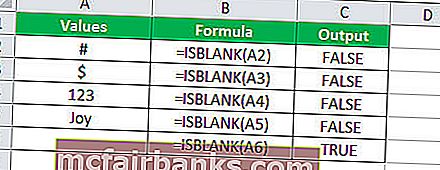
Ячейка A6 пуста и не имеет никакого значения, поэтому она вернула ИСТИННОЕ значение.

Пример # 2

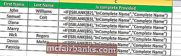
У нас есть список имен с указанием их имени и фамилии, однако есть некоторые имена, для которых фамилия не указана. Нам нужно выяснить, используя формулу Excel, имена, которые являются неполными или без фамилии.

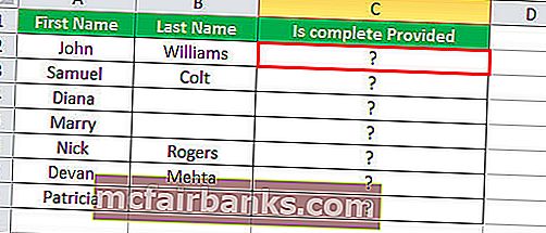
Мы можем использовать эту функцию, чтобы проверить, указана ли фамилия или нет. Если фамилия пуста, функция ISBLANK вернет значение ИСТИНА, используя это значение и функцию ЕСЛИ, мы проверим, указаны ли оба имени или нет.

Формула ISBLANK, которую мы будем использовать:

= ЕСЛИ (ISBLANK (B2), «Неполное имя», «Полное имя»)

Он возвращает значение с использованием ISBLANK, если значение истинно, тогда фамилия не указана, иначе предоставляется фамилия.

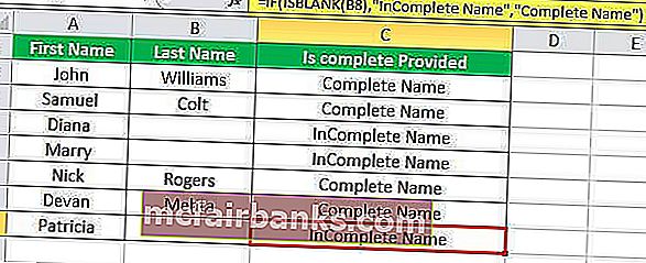
Применяя формулу ISBLANK к остальным ячейкам, которые у нас есть,

Выход:

Пример # 3

Предположим, у нас есть набор данных в диапазоне, показанном ниже:

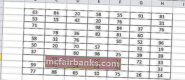
Мы хотим выделить пустые ячейки, например, нам нужно выделить ячейки B5, C4 и другие аналогичные пустые ячейки в диапазоне данных.

Чтобы выделить ячейки, мы будем использовать условное форматирование и функцию ISBLANK.

Мы выберем диапазон из B2: H11, а затем на вкладке Главная мы выберем условное форматирование в Excel ( Главная -> Стили -> Условное форматирование)

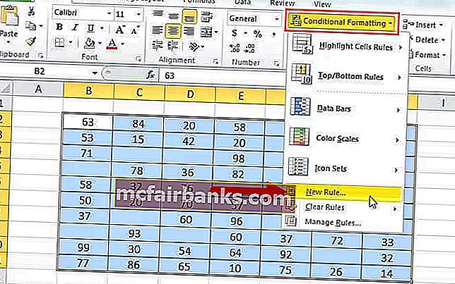
Затем мы выберем Новое правило, и появится всплывающее окно Новое правило форматирования. Мы будем использовать формулу, чтобы определить ячейки для форматирования. Формула ISBLANK, которую мы будем использовать:

= ISBLANK (B2: H11)

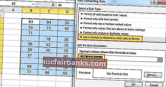
Затем мы выберем формат, выберем цвет выделения и нажмем ОК.

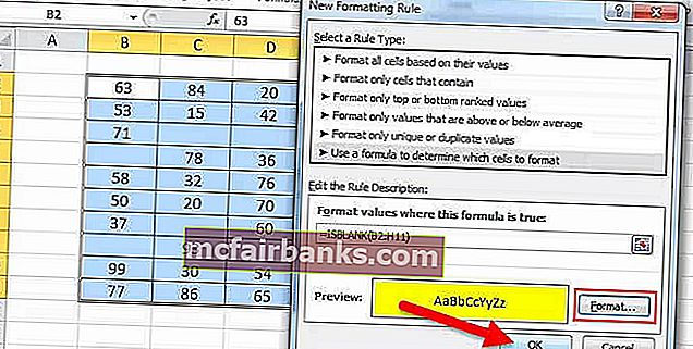
Выход:

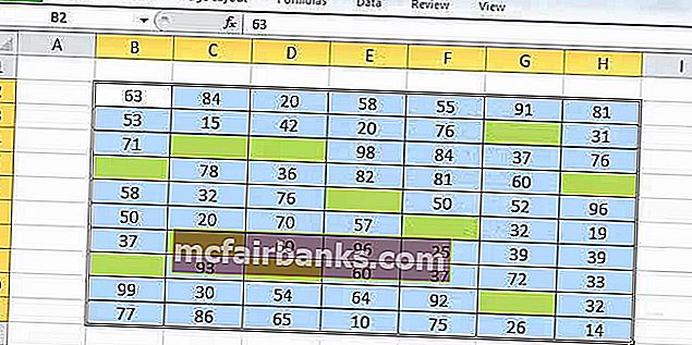
Пример # 4

Различайте пустую ячейку и ячейку, содержащую пустую строку.

У нас есть значения в столбце A. Диапазон A5 содержит пустую строку, а A4 — пустую ячейку. В Excel обе ячейки A4 и A5 кажутся пустыми, но нам нужно определить, является ли это пустой ячейкой или нет.

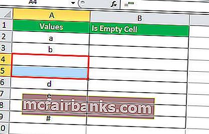
Для этого мы будем использовать функцию ISBLANK и функцию IF для проверки, потому что для пустой строки функция ISBLANK возвращает значение FALSE, она возвращает TRUE только тогда, когда ячейка полностью пуста или равна нулю.

Формула ISBLANK, которую мы будем использовать:

= ЕСЛИ (ISBLANK (A2), «Пусто», «Не пусто»)

Применяя формулу ISBLANK к другим ячейкам, которые у нас есть,

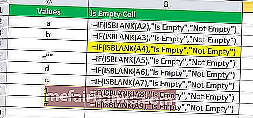
Для ячейки A4 он вернул значение ИСТИНА, следовательно, это пустая ячейка, а в других ячейках есть некоторые, поэтому ISBLANK в excel возвращает для них значение ЛОЖЬ.

Выход:

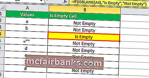
Если в ячейке есть пустая строка («»), функция ISBLANK в excel вернет FALSE, поскольку они не пустые.

Пример # 5

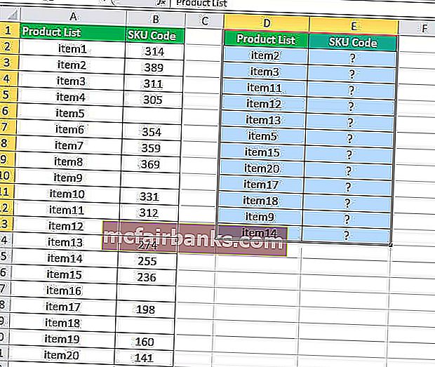
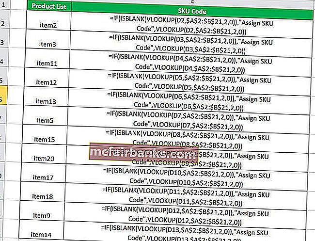
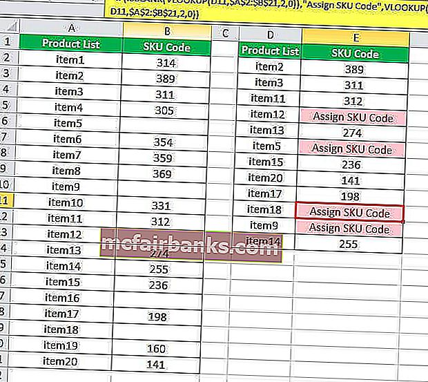
Предположим, у нас есть список товаров с их кодами SKU, а товары, которым не присвоены коды SKU, оставлены пустыми. Столбец A содержит список товаров, а столбец B содержит код SKU, включая товары, для которых коды SKU не были назначены. В столбце D у нас есть некоторый список товаров, не упорядоченных по порядку, и нам нужно найти код SKU, иначе, если код SKU не назначен, мы должны написать формулу, которая может вернуть «Назначить код SKU».

Итак, формула ISBLANK, которую мы будем использовать для выполнения нашего требования, будет

= IF (ISBLANK (VLOOKUP (D2; $ A $ 2: $ B $ 21,2,0)), «Назначить код SKU», VLOOKUP (D2, $ A $ 2: $ B $ 21,2,0))

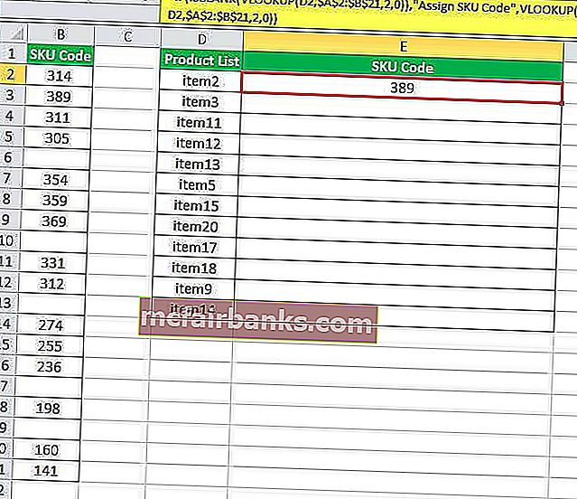
Применяя формулу ISBLANK к другим ячейкам, которые у нас есть,

Выход:

Original text

Contribute a better translation

Источник

You may have a range of data in Excel and need to determine whether or not a cell is Blank. This article explains how to accomplish this using the IF function.

Determine if a cell is blank or not blank

Generally, the Excel IF function evaluates where a cell is Blank or Not Blank to return a specified value in TRUE or FALSE arguments. Moreover, IF function also tests blank or not blank cells to control unexpected results while making comparisons in a logical_test argument or making calculations in TRUE/FALSE arguments because Excel interprets blank cell as zero, and not as an empty or blank cell.

Syntax of IF function is;

IF(logical_test, value_if_true, value_if_false)

In IF statement to evaluate whether the cell is Blank or Not Blank, you can use either of the following approaches;

Logical expressions Equal to Blank (=””) or Not Equal to Blank (<>””)

ISBLANK function to check blank or null values. If a cell is blank, then it returns TRUE, else returns FALSE.

Following examples will explain the difference to evaluate Blank or Not Blank cells using IF statement.

Blank Cells

To evaluate the cells as Blank, you need to use either logical expression Equal to Blank (=””) of ISBLANK function inthe logical_test argument of the IF formula. In both methods logical_test argument returns TRUE if a cell is Blank, otherwise, it returns FALSE if the cell is Not Blank

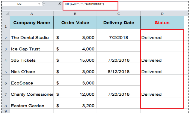
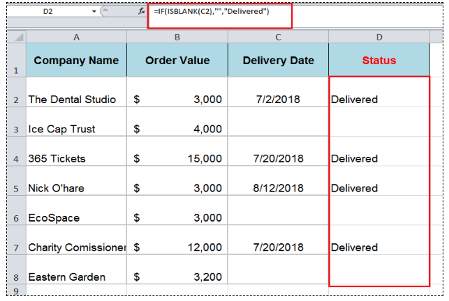
For example, you need to evaluate that if a cell is Blank, the blank value, otherwise return a value “Delivered”. In both approaches, following would be the IF formula;

=IF(C2="","","Delivered")

=IF(ISBLANK(C2),"","Delivered")

In both of the approaches, logical_test argument returns TRUE if a cell is Blank, and the value_if_true argument returns the blank value. Otherwise, the value_if_falseargument returns value “Delivered”.

Not Blank Cells

To evaluate the cells are Not Blank you need to use either the logical expression Not Equal to Blank (<>””) of ISBLANK function in logical_test argument of IF formula. In case of logical expression Not Equal to Blank (<>””) logical_test argument returns TRUE if the cell is Not Blank, otherwise, it returns FALSE. In case of the ISBLANK function, the logical_test argument returns FALSE if a cell is Not Bank. Otherwise it returns TRUE if a cell is blank.

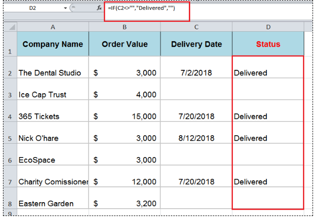
For example, you need to evaluate that if a cell is Not Blank, then return a value “Delivered”, otherwise return a blank value. In both approaches, following would be the IF formula;

=IF(C2<>"","Delivered","")

In this approach, the logical expression Not Equal to Blank (<>“”) returns TRUE in thelogical_test argument if a cell is Not Blank, and the value_if_true argument returns a value “Delivered”, otherwise value_if_false argument a blank value.

=IF(ISBLANK(C2),"","Delivered")

This approach is opposite to first one above. In IF formula, ISBLANK function returns FALSE in thelogical_test argument if a cell is Not Blank, so value_if_true argument returns blank value and a value_if_false argument returns a value “Delivered”.

Still need some help with Excel formatting or have other questions about Excel? Connect with a live Excel expert here for some 1 on 1 help. Your first session is always free.

Are you still looking for help with the IF function? View our comprehensive round-up of IF function tutorials here.

Источник