Formula in excel for blank cells

Bottom Line: In this post we look at 3 ways to copy down values in blank cells in a column.  The techniques include using a formula, Power Query, and a VBA macro.

Skill Level: Intermediate

Watch the Tutorial

Download the Excel Files

You can download both the BEGIN and FINAL files if you want to follow along and practice.

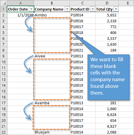
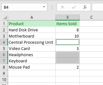
Filling Down Blank Cells

Excel makes it easy to fill down, or copy down, a value into the cells below. You can simply double-click or drag down the fill handle for the cell that you want copied, to populate the cells below it with the same value.

But is there an easy way to replicate that process hundreds of times for reports that have large amounts of data?

In this post we’ll look at three ways to automate this process with: a simple formula, Power Query, and a VBA macro.

1. Filling Down Using a Formula

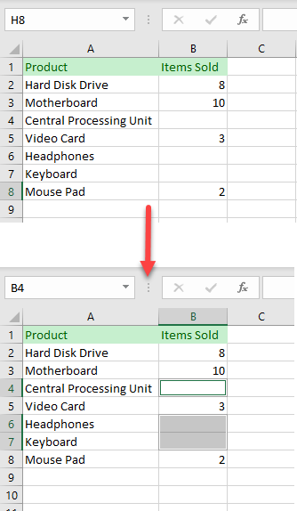
The first way to solve this problem is by using a very simple formula in all of the blank cells that references the cell above. Here are the steps.

Step 1: Select the Blank Cells

In order to select the blank cells in a column and fill them with a formula, we start by selecting all of the cells (including the populated cells). There are many ways to do this, including holding the Shift key down while you navigate to the bottom of your column, or if your data is in an Excel Table, using the keyboard shortcut Ctrl+Space.

Checkout my posts on 7 Keyboard Shortcuts for Selecting Cells and Ranges in Excel and 5 Keyboard Shortcuts for Rows and Columns in Excel to learn more.

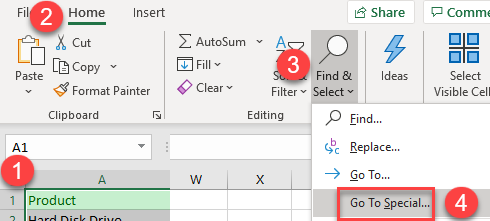
With all of those cells selected, we can pare down our selection to include only the blank cells. This is done by using the Go To Special window from the Find & Select menu on the Home tab of the ribbon.

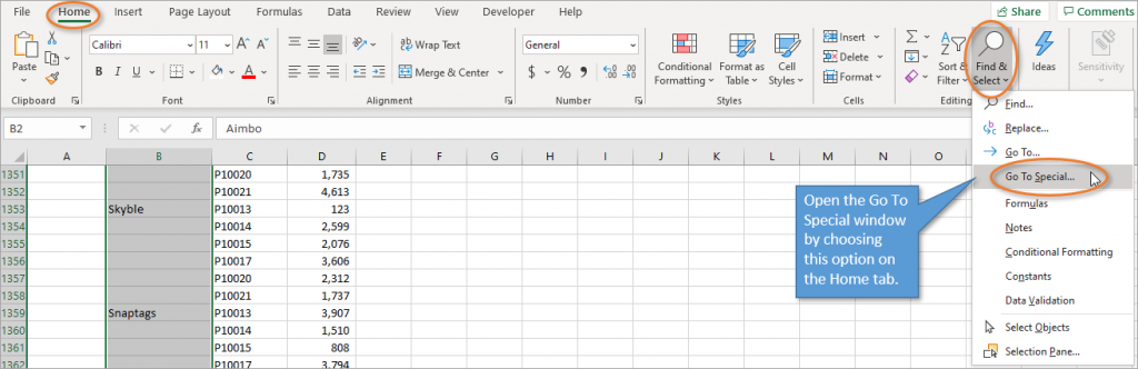
An alternative is to open the Go To window using F5 or Ctrl+G. Then press the Special button for the Go To Special window.

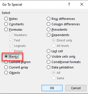
Once the Go To Special window is open, you can choose the option that says Blanks. This will select only the blank cells from the current selection.

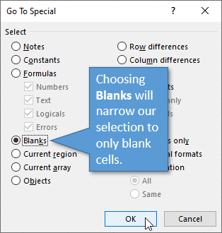
When you hit OK, you’ll notice that the cells that have values in them are no longer selected.

Step 2: Write the Formula

From here you can start typing the formula, which is very simple. Type the equals sign (=) and then reference the cell above (in the case of our example, B2). That’s all you need for the formula!

Step 3: Ctrl+Enter the Formula

After writing the formula, don’t just hit Enter. Instead, use Ctrl+Enter to fill all of the selected cells with the same formula. Hold the Ctrl key, then hit Enter.

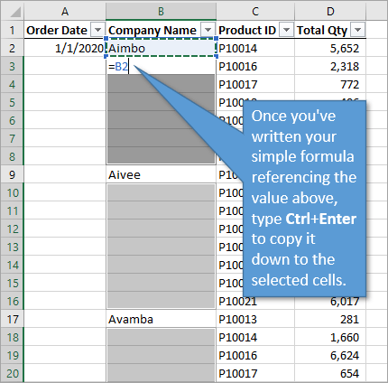
Because your formula reference is relative (B2), not absolute ($B$2), each cell will simply copy the value for the cell directly above it.

Step 4: Copy & Paste Values

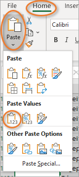
It is a good idea to now copy the entire data column and then paste over it using the Paste Values option so that the data is hard coded. Then, if you do any sorting, the data will not change. You can find the Paste Values option on the Home tab in the Paste drop-down menu:

There are other ways to paste values, including the right-click menu or using keyboard shortcuts. These posts explain those options:

Paste Values with the Right-click & Drag Mouse Shortcut

5 Keyboard Shortcuts to Paste Values in Excel

2. Filling Down Using Power Query

For this option, your data should be in Excel Table format. From anywhere inside the table, you can select the Data or Power Query tab, and then select From Table/Range. You can also create a query that connects to a different data source like a database or the web.

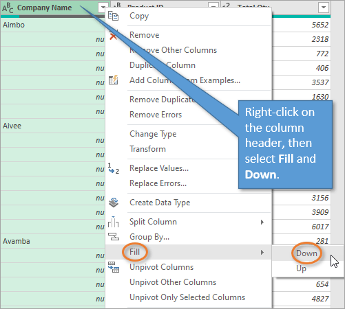
This opens up the Power Query Editor. In Power Query, the blank cells are labeled as null in each cell.

To fill down, just right-click on the column header and select Fill and then Down.

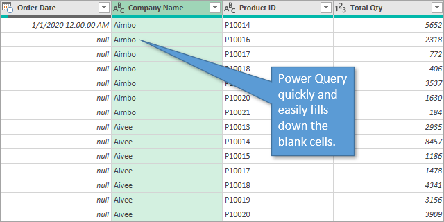
Power Query will fill down each section of blank cells in the column with the value from the cell above it.

When you click on Close & Load, a new sheet will be added to the workbook with these changes.

This process of filling down can be done for multiple columns simultaneously by first selecting multiple columns with Ctrl or Shift, then performing the Fill > Down operation.

If Power Query is somewhat new to you, I invite you to check out this post: Power Query Overview: An Introduction to Excel’s Most Powerful Data Tool.

Free Webinar on Power Query, VBA, & More

I also have a free webinar running right now that covers an introduction to Power Query and the other Excel tools like Power Pivot, Power BI, Macros & VBA, pivot tables, and more.

Click here to register for the webinar

3. Filling Down Using a Macro

To fill down using a macro, start by opening the VB Editor. You can do this by going to the Developer tab and clicking on the Visual Basic button or by using the keyboard shortcut Alt+F11. Insert a new code module, and then write your macro.

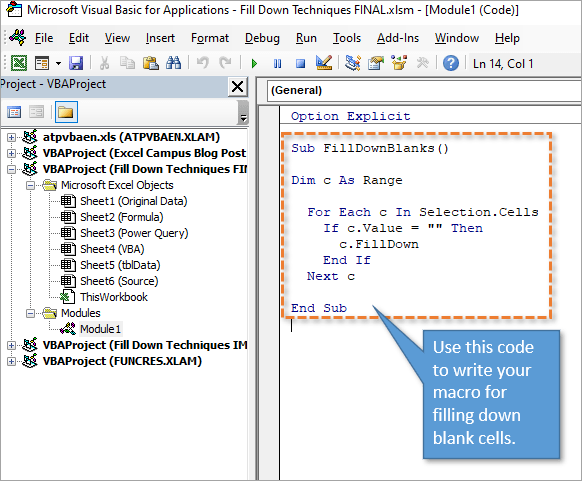
This macro loops through all of the cells in the selected range and performs the FillDown method if the cell is blank. The FillDown method copies the value from the cell above.

If this is a macro that you could use frequently, you might want to consider adding this macro to your personal Macro Workbook and creating a customized button for it. That’s what I’ve done and it looks like this on my Ribbon.

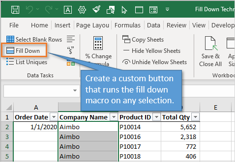
For instruction on how to create a Personal Macro Workbook and custom Ribbon buttons, check out this tutorial: How to Create a Personal Macro Workbook (Video Series).

Pros and Cons

So which of these three methods are right for you? Consider these things:

1. The formula method is simple and easy to implement. It can be done without any knowledge of Power Query or VBA. However, it’s not as quick as a one-click button solution.
2. Power Query requires source data that outputs into a separate worksheet, so it’s more of a process than simply filling down blank cells. If you are already data cleansing on a regular basis for other things, adding this to your existing process might make more sense.
3. Once the initial macro is set up, VBA is a quick solution that’s easy to use—just click a button. However, there is a big disadvantage of this method. You aren’t able to undo your action once that button has been pushed, so you would have to be sure to save a backup copy beforehand if that is a concern for you.

Conclusion

There are three different methods for a very common Excel task. Did I miss any? Please leave a comment below if you have another way to go about it, or have any questions. Thanks! 🙂

The logical expression =»» means «is empty». In the example shown, column D contains a date if a task has been completed. In column E, a formula checks for blank cells in column D. If a cell is blank, the result is a status of «Open». If the cell contains value (a date in this case, but it could be any value) the formula returns «Closed».

The effect of showing «Closed» in light gray is accomplished with a conditional formatting rule.

Display nothing if cell is blank

To display nothing if a cell is blank, you can replace the «value if false» argument in the IF function with an empty string («») like this:

=IF(D5="","","Closed")

Alternative with ISBLANK

Excel contains a function made to test for blank cells called ISBLANK. To use the ISBLANK, you can revise the formula as follows:

=IF(ISBLANK(D5),"Open","Closed")

If the return cell in an Excel formula is empty, Excel by default returns 0 instead. For example cell A1 is blank and linked to by another cell. But what if you want to show the exact return value – for empty cells as well as 0 as return values? This article introduces three different options for dealing with empty return values.

Option 1: Don’t display zero values

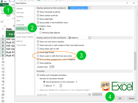
Probably the easiest option is to just not display 0 values. You could differentiate if you want to hide all zeroes from the entire worksheet or just from selected cells.

There are three methods of hiding zero values.

1. Hide zero values with conditional formatting rules.
2. Blind out zeros with a custom number format.
3. Hide zero values within the worksheet settings.

For details about all three methods of just hiding zeroes, please refer to this article.

One small advice on my own account: My Excel add-in “Professor Excel Tools” has a built-in Layout Manager. With this, you can apply this formatting easily to a complete Excel workbook.

Give it a try? Click here and the download starts right away.

Option 2: Change zeroes to blank cells

Unlike the first option, the second option changes the output value. No matter if the return value is 0 (zero) or originally a blank cell, the output of the formula is an empty cell. You can achieve this using the IF formula.

Say, your lookup formula looks like this: =VLOOKUP(A3,C:D,2,FALSE)  (hereafter referred to by “original formula”). You want to prevent getting a zero even if the return value―found by the VLOOKUP formula in column D―is an empty value. This can be achieved using the IF formula.

The structure of such IF formula is shown in the image above (if you need assistance with the IF formula, please refer to this article). The original formula is wrapped within the IF formula. The first argument compares if the original formula returns 0. If yes―and that’s the task of the second argument―the formula returns nothing through the double quotation marks. If the orgininal formula within the first argument doesn’t return zero, the last argument returns the real value. This is achieved by the original formula again.

The complete formula looks like this.

=IF(VLOOKUP(A3,C:D,2,FALSE)=0,"",VLOOKUP(A3,C:D,2,FALSE))

Option 3: Show zeroes but don’t show blank or empty return values

The previous option two didn’t differentiate between 0 and empty cells in the return cell. If you only want to show empty cells if the return cell found by your lookup formula is empty (and not if the return value really is 0) then you have to slightly alter the formula from option 2 before.

Like before, the IF formula is wrapped around the original formula. But instead of testing if the return value is 0, it tests within the first argument if the return value is blank. This is done by the double quotation marks. The rest of the formula is the as before: With the second argument you define that—if the value from the original formula is blank—the return value is empty too. If not, the last argument defines that you return the desired non-blank value.

The formula in your example from option 2 looks like this.

=IF(VLOOKUP(A3,C:D,2,FALSE)="","",VLOOKUP(A3,C:D,2,FALSE))

Option 4: Use Professor Excel Tools to insert the IF functions very quickly

To save some time, we have included a feature for showing blank cells (instead of zeros) in our Excel add-in Professor Excel Tools.

It’s very simple:

1. Select the cells that are supposed to return blanks (instead of zeros).
2. Click on the arrow under the “Return Blanks” button on the Professor Excel ribbon and then on either
   1. Return blanks for zeros and blanks or
   2. Return zeros for zeros and blanks for blanks.

Professor Excel then inserts the IF function as shown in options 2 and 3 above.

Option 5: One elegant solution for not returning zero values…

… was written in the comments. Thanks, Dom! Great to get such awesome feedback from you!

It’s actually quite straight forward: Add two quotation marks in front or after the function and concatenate it with the “&”-character. So, in this case the VLOOKUP function from above would look like this:

=""&VLOOKUP(A3,C:D,2,FALSE)

But: There is a downside. This method forces the cell to a text / string value. This might cause problems in further calculations if a zero is returned. Let me give you an example:

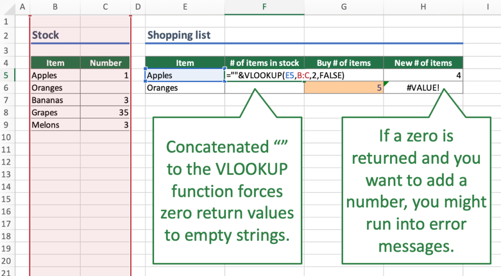
Careful: Return value is interpretated as text.Your VLOOKUP function above is concatenated to an empty string “”. If your return value is 0, the cell will be shown as an empty string. Further calculations might be difficult: For example, if you want to add a number to the return value. Referring directly to the cell, for example =F6+G6 leads to the #VALUE error message as shown above. However, using the SUM function =SUM(F6,G6) still works.

Bottom line: This is an elegant approach, but please test it well if it suits to your Excel model.

Image by Pexels from Pixabay

Sometimes you need to check if a cell is blank, generally because you might not want a formula to display a result without input.

In this case we’re using IF with the ISBLANK function:

• =IF(ISBLANK(D2),»Blank»,»Not Blank»)

Which says IF(D2 is blank, then return «Blank», otherwise return «Not Blank»). You could just as easily use your own formula for the «Not Blank» condition as well. In the next example we’re using «» instead of ISBLANK. The «» essentially means «nothing».

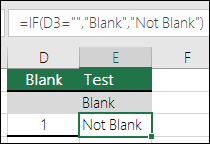
=IF(D3=»»,»Blank»,»Not Blank»)

This formula says IF(D3 is nothing, then return «Blank», otherwise «Not Blank»). Here is an example of a very common method of using «» to prevent a formula from calculating if a dependent cell is blank:

• =IF(D3=»»,»»,YourFormula())

  IF(D3 is nothing, then return nothing, otherwise calculate your formula).

See all How-To Articles

In this tutorial, you will learn how to find blank cells in Excel and Google Sheets.

Find & Select Empty Cells

There is an easy way to select all the blank cells in any selected range in Excel. Although this method won’t show you the number of blank cells, it will highlight all of them so you can easily locate them in a spreadsheet.

1. First, select the entire data range. Then in the Ribbon, go to Home > Find & Select > Go To Special.

2. In Go To Special dialog window click on Blanks and when done press OK.

As a result, all blank cells are selected.

With this method, you won’t find pseudo-blank cells (cells with formulas that return blanks and cells containing only spaces).

Other ways to identify blanks:

• IsEmpty Function in VBA
• How to use the ISBLANK Function

Find Blank Cells in Google Sheets

Unlike Excel, Google Sheets doesn’t have a Go To Special feature. But you can identify blank cells and select them one-by-one, highlight them, or replace them.