
Total the data in an Excel table
You can quickly total data in an Excel table by enabling the Total Row option, and then use one of several functions that are provided in a drop-down list for each table column. The Total Row default selections use the SUBTOTAL function, which allow you to include or ignore hidden table rows, however you can also use other functions.

-
Click anywhere inside the table.
-
Go to Table Tools > Design, and select the check box for Total Row.

-
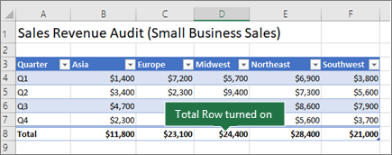
The Total Row is inserted at the bottom of your table.
Note: If you apply formulas to a total row, then toggle the total row off and on, Excel will remember your formulas. In the previous example we had already applied the SUM function to the total row. When you apply a total row for the first time, the cells will be empty.
-
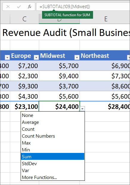
Select the column you want to total, then select an option from the drop-down list. In this case, we applied the SUM function to each column:
You’ll see that Excel created the following formula: =SUBTOTAL(109,[Midwest]). This is a SUBTOTAL function for SUM, and it is also a Structured Reference formula, which is exclusive to Excel tables. Learn more about Using structured references with Excel tables.
You can also apply a different function to the total value, by selecting the More Functions option, or writing your own.
Note: If you want to copy a total row formula to an adjacent cell in the total row, drag the formula across using the fill handle. This will update the column references accordingly and display the correct value. If you copy and paste a formula in the total row, it will not update the column references as you copy across, and will result in inaccurate values.

You can quickly total data in an Excel table by enabling the Total Row option, and then use one of several functions that are provided in a drop-down list for each table column. The Total Row default selections use the SUBTOTAL function, which allow you to include or ignore hidden table rows, however you can also use other functions.
-
Click anywhere inside the table.
-
Go to Table > Total Row.
-
The Total Row is inserted at the bottom of your table.
Note: If you apply formulas to a total row, then toggle the total row off and on, Excel will remember your formulas. In the previous example we had already applied the SUM function to the total row. When you apply a total row for the first time, the cells will be empty.
-
Select the column you want to total, then select an option from the drop-down list. In this case, we applied the SUM function to each column:
You’ll see that Excel created the following formula: =SUBTOTAL(109,[Midwest]). This is a SUBTOTAL function for SUM, and it is also a Structured Reference formula, which is exclusive to Excel tables. Learn more about Using structured references with Excel tables.
You can also apply a different function to the total value, by selecting the More Functions option, or writing your own.
Note: If you want to copy a total row formula to an adjacent cell in the total row, drag the formula across using the fill handle. This will update the column references accordingly and display the correct value. If you copy and paste a formula in the total row, it will not update the column references as you copy across, and will result in inaccurate values.
You can quickly total data in an Excel table by enabling the Toggle Total Row option.
-
Click anywhere inside the table.
-
Click the Table Design tab > Style Options > Total Row.
The Total row is inserted at the bottom of your table.
Set the aggregate function for a Total Row cell
Note: This is one of several beta features, and currently only available to a portion of Office Insiders at this time. We’ll continue to optimize these features over the next several months. When they’re ready, we’ll release them to all Office Insiders, and Microsoft 365 subscribers.
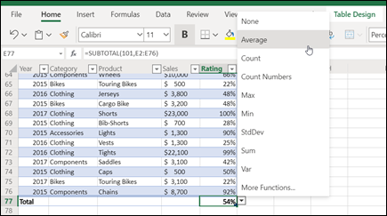
The Totals Row lets you pick which aggregate function to use for each column.
-
Click the cell in the Totals Row under the column you want to adjust, then click the drop-down that appears next to the cell.
-
Select an aggregate function to use for the column. Note that you can click More Functions to see additional options.
Need more help?
You can always ask an expert in the Excel Tech Community or get support in the Answers community.
See Also
Overview of Excel tables
Video: Create an Excel table
Create or delete an Excel table
Format an Excel table
Resize a table by adding or removing rows and columns
Filter data in a range or table
Convert a table to a range
Using structured references with Excel tables
Subtotal and total fields in a PivotTable report
Subtotal and total fields in a PivotTable
Excel table compatibility issues
Export an Excel table to SharePoint
Need more help?
Want more options?
Explore subscription benefits, browse training courses, learn how to secure your device, and more.
Communities help you ask and answer questions, give feedback, and hear from experts with rich knowledge.
You’re likely going to come across the need for running totals if you’re dealing with any sort of daily data.
Imagine you track sales each day. Your data contains a row for each date with a total sales amount, but maybe you want to know the total sales for the month at each day. This is a running total, it’s the sum of all sales up to and including the current days sales.
In this post we’ll cover multiple ways to calculate a running total for your daily data. We’ll explore how to use worksheet formulas, pivot tables, power pivot with DAX and power query.
We’ll also explore what happens to the running total calculation when inserting or deleting rows of data and how to update the results.
Get the file with all the examples.
Running Totals with a Simple Formula
It’s possible to create a basic running total formula using the + operator.
However, we’ll need to use two different formulas to get the job done.
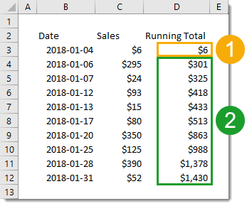
- =C3 will be the first formula and will only be in the first row of the running total.
- =C4+D3 will be in the second row and can be copied down the remaining rows for the running total.
The formula in our first row can’t add the cell above it to the total as it contains a text value for a column heading. This would cause a #VALUE! error to appear in the running total since the + can’t handle text values. We avoid this with a different formula in the first row which doesn’t reference the cell above.
What happens to the running total when we insert or delete rows in our data?
Inserting a new row will result in a gap in the running total. To fix this, we’ll need to copy the formula down from the first cell above the newly inserted rows all the way down to the last row.
Deleting any rows will result in #REF! errors since deleting a row means deleting a cell referenced by the formula below it. To fix this, we’ll need to copy the formula down from the last error-free cell all the way down to the last row.
Running Totals with a SUM Formula
We can avoid the awkwardness of using two different formulas in our running total column by utilizing the SUM function instead of the + operator. When the SUM function encounters a text cell it will treat it the same as a though it contained a 0.
This way we can use the following formula uniformly for every row including the first row.
=SUM(C3,D2)
This formula will reference the column heading containing text for the first row, but this ok as it’s treated like a 0.
When inserting or deleting rows, we will still encounter the same problems with blank cells and errors. We can fix them the same way as with running totals in the simple formula method.
Running Totals with a Partially Fixed Range
Another option with the SUM function is to only reference the Sales column and use a partially fixed range reference.
If we use the following formula =SUM($C$3:C3), we can copy and paste this down the range. It won’t reference any column headings and the range referenced will grow to each row.
Unfortunately, this too will have the same problems (and solutions) with inserting or deleting rows.
Running Totals with a Relative Named Range
We can avoid the problems with inserting and deleting rows from our data if we use a relative named range. This will refer to the cell directly above no matter how many rows we insert or delete.
This is a trick that involves temporarily switching the Excel reference style from A1 to R1C1. Then defining a named range using the R1C1 notation. Then switching the reference style back to A1.
In R1C1 reference style, cells are referred to by how far away they are from the cell using the reference. For example, =R[-2]C[3] refers to the cell 2 up and 3 to the right of the cell using this formula.
We can use this relative referencing to create a named range that’s always one cell above the referring cell with the formula =R[-1]C.
To switch reference style, go to the File tab then choose Options. Go to the Formula section in the Excel Options menu and check the R1C1 reference style box and then press the OK button.
Now we can add our named range. Go to the Formula tab of the Excel ribbon and choose the Define Name command.
Insert a name like “Above” as the name of the range. Add the formula =R[-1]C into the Refers to input and press the OK button.
We can now switch Excel back to the default reference style. Go to the File tab > Options the Formula section > uncheck the R1C1 reference style box > then press the OK button.
Now we can use the formula =SUM([@Sales],Above) in our running total column.
The named range Above will always refer to the cell directly above. When we insert or delete rows, the relative named range will adjust accordingly and no action is needed.
In fact if we place our data in an Excel Table then the formula will automatically fill down for any new rows since the formula is uniform for the entire column. No action is needed to copy down any formulas.
Running Totals with a Pivot Table
Pivot tables are super useful for summarizing any type of data. There’s more to them than just adding, counting and finding averages. There are many other types of calculations built in, and there is actually a running total calculation!
First, we need to insert a pivot table based on the data. Select a cell inside the data and go to the Insert tab and choose the PivotTable command. Then go through the Create PivotTable window to choose where you want the pivot table, either in a new worksheet or somewhere in an existing one.
Add the Date field into the Rows area of the pivot table, then add the Sales field into the Values area of the pivot table. Now add another instance of the Sales field into the Rows area.
We should now have two identical Sales fields with one of them being labelled Sum of Sales2. We can rename this label anytime by simply typing over it with something like Running Total.
Right click on any of the values in the Sum of Sales2 field and select Show Value As then choose Running Total In.
We want to show the running total by date, so in the next window we need to select Date as the Base Field.
That’s it, we now have a new calculation which displays the running total of our sales inside the pivot table.
What happens if we add or delete a row in our source data, how does this affect the running total? The pivot table calculations are dynamic and will take any new data into account in its running total calculation, we will just need to refresh the pivot table.
Right click anywhere inside the pivot table and choose Refresh from the menu.
Running Totals with Power Pivot and DAX Measures
The first couple steps for this are the exact same using a regular pivot table.
Select a cell inside the data and go to the Insert tab and choose the PivotTable command.
When you come to the Create PivotTable menu, check the Add this data to the Data Model box to add the data to the data model and enable it for use with power pivot.
Place the Date field in the Rows area and the Sales field in the Values area of the pivot table.
With power pivot, we will need to create any extra calculations we want using the DAX language. Right click on the table name in the PivotTable Fields window, then select Add Measure to create a new calculation. Note, this is only available with the data model.
=CALCULATE (
    SUM ( Sales[Sales] ),
    FILTER (
        ALL (Sales[Date] ),
        Sales[Date] <= MAX (Sales[Date])
    )
)
Now we can create our new running total measure.
- In the Measure window, we need to add a Measure Name. In this case we can name the new measure as Running Total.
- We also need to add the above formula into the Formula box.
- The cool thing about power pivot is the ability to assign a number format to a measure. We can choose the Currency format for our measure. Whenever we use this measure in a pivot table the format will automatically be applied.
Press the OK button and the new measure will be created.
There will be a new field listed in the PivotTable Fields window. It has a small fx icon on the left to denote that it’s a measure and not a regular field in the data.
We can use this new field just like any other field and drag it into the Values area to add our running total calculation into the pivot table.
What happens to the running total when we add or remove data from the source table? Just like a regular pivot table, we simply need to right click on the pivot table and select Refresh to update the calculation.
Running Totals with a Power Query
We can also add running totals to our data using power query.
First we need to import the table into power query. Select the table of data and go to the Data tab and choose the From Table/Range option. This will open the power query editor.
Next we can sort our data by date. This is an optional step we can add so that if we change the order of our source data, the running total will still appear by date.
Click on the filter toggle in the date column heading and choose Sort Ascending from the options.
We need to add an index column. This will be used in the running total calculation later on. Go to the Add Column tab and click on the small arrow next to the Index Column to insert an index starting at 1 in the first row.
We need to add a new column to our query to calculate the running total. Go to the Add Column tab and choose the Custom Column command.
We can name the column as Running Total and add the following formula.
List.Sum(List.Range(#"Added Index"[Sales],0,[Index]))
The List.Range function creates a list of values from the Sales column starting at the 1st row (0th item) which spans a number of rows based on the value in the index column.
The List.Sum function then adds up this list of values which is our running total.
We no longer need the index column, it has served its purpose and we can remove it. Right click on the column heading and select Remove from the options.
We’ve got our running total and are finished with the query editor. We can close the query and load the results into a new worksheet. Go to the Home tab of the query editor and press the Close & Load button.
What happens with the running total when we add or remove rows from our source data? We will need to refresh the power query output table to update the running total with the changes. Right click anywhere on the table and choose Refresh to update the table.
With the optional sorting step above, if we add dates out of order to the source data, power query will sort by date and return the correct order by date for the running total.
Conclusions
There are many different options for calculating running totals in Excel.
We’ve explored options including formulas in the worksheet, pivot tables, power pivot DAX formulas, and power query. Some offer a more robust solution when adding or removing rows from the data, other methods offer an easier implementation.
Simple formulas in the worksheet are easy to set up but won’t handle inserting or deleting new rows of data easily. Other solutions like pivot tables, DAX and power query are more robust and handle inserting or deleting rows of data easily but are harder to set up.
It’s good to be aware of the pros and cons of each method and choose the one best suited. If you won’t be inserting or deleting new data, then worksheet formulas might be the way to go.
About the Author
John is a Microsoft MVP and qualified actuary with over 15 years of experience. He has worked in a variety of industries, including insurance, ad tech, and most recently Power Platform consulting. He is a keen problem solver and has a passion for using technology to make businesses more efficient.
Asked by: Sharon Olson
Score: 4.3/5
(35 votes)
Enter the SUM function manually to sum a column In Excel
- Click on the cell in your table where you want to see the total of the selected cells.
- Enter =sum( to this selected cell.
- Now select the range with the numbers you want to total and press Enter on your keyboard. Tip.
What is the formula of sum in Excel?
The SUM function adds values. You can add individual values, cell references or ranges or a mix of all three. For example: =SUM(A2:A10) Adds the values in cells A2:10.
How do I total a sum in Excel?
To sum a range of cells, use the SUM function. To sum cells based on one criteria (for example, greater than 9), use the following SUMIF function (two arguments). To sum cells based on one criteria (for example, green), use the following SUMIF function (three arguments, last argument is the range to sum).
How do I sum an entire column in Excel?
To add up an entire column, enter the Sum Function: =sum( and then select the desired column either by clicking the column letter at the top of the screen or by using the arrow keys to navigate to the column and using the CTRL + SPACE shortcut to select the entire column. The formula will be in the form of =sum(A:A).
How do you add up cells in Excel?
AutoSum makes it easy to add adjacent cells in rows and columns. Click the cell below a column of adjacent cells or to the right of a row of adjacent cells. Then, on the HOME tab, click AutoSum, and press Enter. Excel adds all of the cells in the column or row.
21 related questions found
How do you create a formula for a column in Excel?
To insert a formula in Excel for an entire column of your spreadsheet, enter the formula into the topmost cell of your desired column and press «Enter.» Then, highlight and double-click the bottom-right corner of this cell to copy the formula into every cell below it in the column.
How do you sum a column and row criteria?
Method 1: Summing up the matching column header and row header Using the SUMPRODUCT function.
- column_headers: It is the header range of columns that you want to sum. …
- row_headers: It is the header range of rows that you want to sum. …
- (C2:N2=B13): This statement will return an array of TRUE and FALSE.
How do you apply formula to entire column in Excel without dragging?
7 Answers
- First put your formula in F1.
- Now hit ctrl+C to copy your formula.
- Hit left, so E1 is selected.
- Now hit Ctrl+Down. …
- Now hit right so F20000 is selected.
- Now hit ctrl+shift+up. …
- Finally either hit ctrl+V or just hit enter to fill the cells.
How do you sum categories in Excel?
Sum values by group with using formula
Select next cell to the data range, type this =IF(A2=A1,»»,SUMIF(A:A,A2,B:B)), (A2 is the relative cell you want to sum based on, A1 is the column header, A:A is the column you want to sum based on, the B:B is the column you want to sum the values.)
How do I enable sum and count in Excel?
Select the range of cells you want to calculate. The sum, average, and count of the selected cells appears on the status bar by default. If you want to change the type of calculations that appear on the Status bar, right-click anywhere on the Status bar to display a shortcut menu.
How do you calculate the average sum in Excel?
AutoSum lets you find the average in a column or row of numbers where there are no blank cells.
- Click a cell below the column or to the right of the row of the numbers for which you want to find the average.
- On the HOME tab, click the arrow next to AutoSum > Average, and then press Enter.
Which formula is not entered correctly?
Solution(By Examveda Team)
A formula always starts with an equal sign (=), which can be followed by numbers, math operators (such as a plus or minus sign), and functions, which can really expand the power of a formula. Here in option D 10+50 there is no equal sign (=), so it is not correct.
How do I do a percentage formula in Excel?
The percentage formula in Excel is = Numerator/Denominator (used without multiplication by 100). To convert the output to a percentage, either press “Ctrl+Shift+%” or click “%” on the Home tab’s “number” group.
How do I apply a formula to an entire column in VBA?
Using the Fill Down Option (it’s in the ribbon)
- In cell A2, enter the formula: =B2*15%
- Select all the cells in which you want to apply the formula (including cell C2)
- Click the Home tab.
- In the editing group, click on the Fill icon.
- Click on ‘Fill down’
How do you sum a column with multiple criteria?
2. To sum with more criteria, you just need to add the criteria into the braces, such as =SUM(SUMIF(A2:A10, {«KTE»,»KTO»,»KTW»,»Office Tab»}, B2:B10)). 3. This formula only can use when the range cells that you want to apply the criteria against in a same column.
How do you sum rows based on criteria?
For example, the formula =SUMIF(B2:B5, «John», C2:C5) sums only the values in the range C2:C5, where the corresponding cells in the range B2:B5 equal «John.» To sum cells based on multiple criteria, see SUMIFS function.
How do you sum a value in a table?
Click the table cell where you want your result to appear. On the Layout tab (under Table Tools), click Formula. In the Formula box, check the text between the parentheses to make sure Word includes the cells you want to sum, and click OK. =SUM(ABOVE) adds the numbers in the column above the cell you’re in.
What is the formula to calculate average?
How to Calculate Average. The average of a set of numbers is simply the sum of the numbers divided by the total number of values in the set. For example, suppose we want the average of 24 , 55 , 17 , 87 and 100 . Simply find the sum of the numbers: 24 + 55 + 17 + 87 + 100 = 283 and divide by 5 to get 56.6 .
What is mode formula?
In statistics, the mode formula is defined as the formula to calculate the mode of a given set of data. Mode refers to the value that is repeatedly occurring in a given set and mode is different for grouped and ungrouped data sets. Mode = L+h(fm−f1)(fm−f1)−(fm−f2) L + h ( f m − f 1 ) ( f m − f 1 ) − ( f m − f 2 )
What is average in math formula?
In maths, the average value in a set of numbers is the middle value, calculated by dividing the total of all the values by the number of values. When we need to find the average of a set of data, we add up all the values and then divide this total by the number of values.
How do I add a formula to existing data in Excel?
Just select all the cells at the same time, then enter the formula normally as you would for the first cell. Then, when you’re done, instead of pressing Enter, press Control + Enter. Excel will add the same formula to all cells in the selection, adjusting references as needed.
Where is the formula on Excel?
See a formula
- When a formula is entered into a cell, it also appears in the Formula bar.
- To see a formula, select a cell, and it will appear in the formula bar.
Which symbol is entered before a formula?
If you type in the formula, you must start with an equal sign, so Excel knows that the data in the cell is a formula. After the =, what comes next depends on what you’re trying to do. If you are multiplying numbers, just type in the appropriate numbers and mathematical symbol (* for multiply).
The SUM function in excel adds the numerical values in a range of cells. Being categorized under the Math and Trigonometry function, it is entered by typing “=SUM” followed by the values to be summed. The values supplied to the function can be numbers, cell references or ranges.
For example, cells B1, B2, and B3 contain 20, 44, and 67 respectively. The formula “=SUM(B1:B3)” adds the numbers of the cells B1 to B3. It returns 131.
The SUM formula automatically updates with the insertion or deletion of a value. It also includes the changes made to an existing cell range. Moreover, the function ignores the empty cells and text values.
Table of contents
- SUM Function in Excel
- The Syntax of the SUM Excel Function
- The Procedure to Enter the SUM Function in Excel
- The AutoSum Option in Excel
- How to Use the SUM Function in Excel?
- Example #1
- Example #2
- Example #3
- Example #4
- Example #5
- The Usage of the SUM Excel Function
- The Limitations of the SUM Function in Excel
- The Nesting of the SUM Excel Function
- Frequently Asked Questions
- SUM Function in Excel Video
- Recommended Articles
The Syntax of the SUM Excel Function
The syntax of the function is shown in the following image:

The function accepts the following arguments:
- Number1: This is the first numeric value to be added.
- Number2: This is the second numeric value to be added.
The “number1” argument is required while the subsequent numbers (“number 2”, “number 3”, etc.) are optional.
The Procedure to Enter the SUM Function in Excel
You can download this SUM Function Excel Template here – SUM Function Excel Template
To enter the SUM function manually, type “=SUM” followed by the arguments.
The alternative steps to enter the SUM excel function are listed as follows:
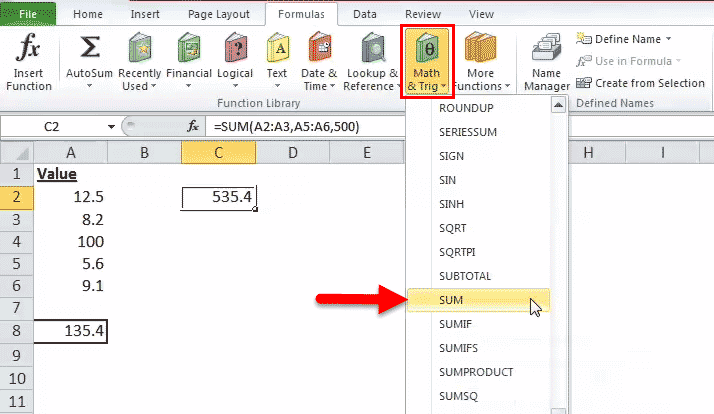
- In the Formulas tab, click the “math & trig” option, as shown in the following image.
2. From the drop-down menu that opens, select the SUM option.
3. In the “function arguments” dialog box, enter the arguments of the SUM function. Click “Ok” to obtain the output.

The AutoSum Option in Excel
The AutoSum option is the fastest way to add numbers in a range of cells. It automatically enters the SUM formula in the selected cell.
Let us work on an example to understand the working of the AutoSum option. We want to sum the list of values in A2:A7, shown in the succeeding image.
The steps to use the AutoSum command are listed as follows:
- Select the blank cell immediately following the cell to be summed up. Choose the cell A8.

- In the Home tab, click “AutoSum”. Alternatively, press the shortcut keys “Alt+=” together and without the inverted commas.

- The SUM formula appears in the selected cell. It shows the reference of the cells that have been summed up.

- Press the “Enter” key. The output appears in cell A8, as shown in the following image.


How to Use the SUM Function in Excel?
Let us consider a few examples to understand the usage of the SUM function. The examples #1 to #5 show an image containing a list of numeric values.
Example #1
We want to sum the cells A2 and A3 shown in the succeeding image.
Apply the formula “=SUM(A2, A3).” It returns 20.7 in cell C2.

Example #2
We want to sum the cells A3, A5, and the number 45 shown in the succeeding image.
Apply the formula “=SUM (A3, A5, 45).” It returns 58.8 in cell C2.

Example #3
We want to sum the cells A2, A3, A4, A5, and A6 shown in the succeeding image.
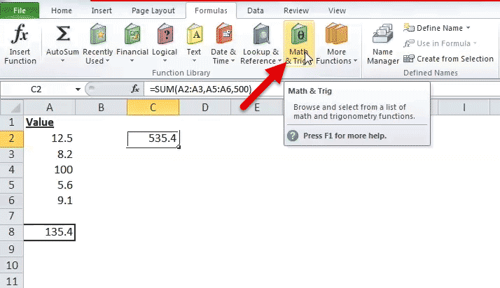
Apply the formula “=SUM (A2:A6).” It returns 135.4 in cell C2.

Example #4
We want to sum the cells A2, A3, A5, and A6 shown in the succeeding image.
Apply the formula “=SUM (A2:A3, A5:A6).” It returns 35.4 in cell C2.

Example #5
We want to sum the cells A2, A3, A5, A6, and the number 500 shown in the succeeding image.
Apply the formula “=SUM (A2:A3, A5:A6, 500).” It returns 535.4 in cell C2.

The Usage of the SUM Excel Function
The rules governing the usage of the function are listed as follows:
- The arguments supplied can be numbers, arrays, cell references, constants, ranges, and the results of other functions or formulas.
- While providing a range of cells, only the first range (cell1:cell2) is required.
- The output is numeric and represents the sum of values supplied.
- The arguments supplied can go up to a total of 255.
Note: The SUM excel function returns the “#VALUE!” error if the criterion supplied is a text string longer than 255 characters.
The Limitations of the SUM Function in Excel
The drawbacks of the function are listed as follows:
- The cell range supplied must match the dimensions of the source.
- The cell containing the output must always be formatted as a number.
The Nesting of the SUM Excel Function
The built-in formulas of Excel can be expanded by nesting one or more functions inside another function. This permits multiple calculations to take place in a single cell of the worksheet.
The nested function acts as an argument of the main or the outermost function. Excel calculates the innermost function first and then moves outwards.
For example, the following formula shows the SUM function nested within the ROUND functionThe ROUNDUP excel function calculates the rounded value of the number to the upward side or the higher side. In other words, it rounds the number away from zero. Being an inbuilt function of Excel, it accepts two arguments–the “number” and the “num_of _digits.” For example, “=ROUNDUP(0.40,1)” returns 0.4.
read more:

For the given formula, the output is calculated as follows:
- First, the sum of the values in cells A1 to A6 is computed.
- Next, the resulting number is rounded to three decimal places.
With Microsoft Excel 2007, nested functions up to 64 levels are permitted. Prior to this version, one could nest functions only till 7 levels.
Frequently Asked Questions
1. Define the SUM function of Excel.
The SUM function helps add the numerical values. These values can be supplied to the function as numbers, cell references, or ranges. The SUM function is used when there is a need to find the total of specified cells.
The syntax of the SUM excel function is stated as follows:
“SUM(number1,[number2] ,…)”
The “number1” and “number2” are the first and second numeric values to be added. The “number1” argument is mandatory while the remaining values are optional.
In the SUM function, the range to be summed can be provided, which is easier than typing the cell references one by one. The AutoSum option provided in the Home or Formulas tab of Excel is the simplest way to sum two numbers.
Note: The numeric value provided as an argument can be either positive or negative.
2. How to sum the values of filtered data in Excel?
To add the values of filtered data, use the SUBTOTAL function. The syntax of the function is stated as follows:
“SUBTOTAL(function_num,ref1,[ref2],…)”
The “function_num” is a number ranging from 1 to 11 or 101 to 111. It indicates the function to be used for the SUBTOTALThe SUBTOTAL excel function performs different arithmetic operations like average, product, sum, standard deviation, variance etc., on a defined range.read more. The functions used can be AVERAGE, MAX, MIN, COUNT, STDEV, SUM, and so on.
The “ref1” and “ref2” are the cells or ranges to be added.
The “function_num” and “ref1” arguments are mandatory. The “function_num” 109 is used for adding the visible cells of filtered data.
Let us consider an example.
• The sales revenue generated by A and B of team X are:
$1,240 and $3,562 given in cells C2 and C3 respectively
• The sales revenue generated by C and D of team Y are:
$2,351 and $4,109 given in cells C4 and C5 respectively
We filter only team X rows and apply the formula “SUBTOTAL(109,C2:C3).” It returns $4,802.
Note: Alternatively, the AutoSum property can be used to sum the filtered cells.
3. State the benefits of using the SUM function in Excel.
The benefits of using the SUM function are listed as follows:
• It helps obtain the totals of ranges irrespective of whether the cells are contiguous or non-contiguous.
• It ignores the empty cells and text values entered in a cell. In such cases, it returns an output representing the sum of the remaining numbers of the range.
• It automatically updates to include the addition of a row or a column.
• It automatically updates to exclude the deletion of a row or column.
• It eliminates the difficulty associated with typing manual entries.
• It makes the output more readable by allowing the cell to be formatted as a number.
SUM Function in Excel Video
Recommended Articles
This has been a guide to the SUM function in Excel. Here we discuss how to use Sum Formula along with step by step examples and FAQs. You can download the Excel template from the website. Take a look at these useful functions of Excel–
- SUMIFS with Multiple Criteria
- SUMX in Power BISUMX is a function in power BI which returns the sum of expression from a table. It is an inbuilt mathematical function. The syntax used for this function is SUMX(,).read more
- TEXT Function
- Concatenate Excel Function
- Excel Alternate Row ColorThe two different methods to add colour to alternative rows are adding alternative row colour using Excel table styles or highlighting alternative rows using the Excel conditional formatting option.read more
Reader Interactions
Return value
The sum of values supplied.
Usage notes
The SUM function returns the sum of values supplied. These values can be numbers, cell references, ranges, arrays, and constants, in any combination. SUM can handle up to 255 individual arguments.
The SUM function takes multiple arguments in the form number1, number2, number3, etc. up to 255 total. Arguments can be a hardcoded constant, a cell reference, or a range. All numbers in the arguments provided are summed. The SUM function automatically ignores empty cells and text values, which makes SUM useful for summing cells that may contain text values.
The SUM function will sum hardcoded values and numbers that result from formulas. If you need to sum a range and ignore existing subtotals, see the SUBTOTAL function.
Examples
Typically, the SUM function is used with ranges. For example:
=SUM(A1:A9) // sum 9 cells in A1:A9
=SUM(A1:F1) // sum 6 cells in A1:F1
=SUM(A1:A100) // sum 100 cells in A1:A100
Values in all arguments are summed together, so the following formulas are equivalent:
=SUM(A1:A5)
=SUM(A1,A2,A3,A4,A5)
=SUM(A1:A3,A4:A5)
In the example shown, the formula in D12 is:
=SUM(D6:D10) // returns 9.05
References do not need to be next to one another. For example:
=SUM(A1,F13,E100)
Sum with text values
The SUM function automatically ignores text values without returning an error. This can be useful in situations like this, where the first formula would otherwise throw an error.
Keyboard shortcut
Excel provides a keyboard shortcut to automatically sum a range of cells above. You can see a demonstration in this video.
Notes
- SUM automatically ignores empty cells and cells with text values.
- If arguments contain errors, SUM will return an error.
- The AGGREGATE function can sum while ignoring errors.
- SUM can handle up to 255 total arguments.
- Arguments can be supplied as constants, ranges, named ranges, or cell references.