
The MONTH function in Excel is a date function used to find the month for a given date in a date format. This function takes an argument in a date format, and the result is in integer format. This function’s value is in the range of 1-12 as there are only twelve months in a year. The method to use this function is as follows =MONTH( serial_number). The argument provided to this function should be in a recognizable date format of Excel.
For example, =MONTH(A1) – returns the month of a date in A1.
=MONTH(DATE(2020,6,10)) – returns 6 corresponding to June.
Also, =MONTH(“10-June-2020”) – returns number 6 too.
The MONTH function in Excel gives the month from its date. It returns the month number ranging from 1 to 12.
Table of contents
- MONTH Function in Excel
- MONTH Formula in Excel
- MONTH in Excel – Illustration
- How to Use MONTH Function in Excel?
- MONTH in Excel Example #1
- MONTH in Excel Example #2
- MONTH in Excel Example #3
- MONTH in Excel Example #4
- MONTH in Excel Example #5
- Things to remember about a MONTH in Excel
- MONTH Excel Function Video
- Recommended Articles
MONTH Formula in Excel
Below is the MONTH Formula in Excel.

Or
MONTH( date )
MONTH in Excel – Illustration
Suppose a date (10 August, 18) is given in cell B3. You want to find the month in Excel of the given date in numbers.

You can use the MONTH formula in Excel given below:
= MONTH (B3)

Press the “Enter” key. The MONTH function in Excel will return 8.

You can also use the following MONTH formula in Excel:
= MONTH (“10 Aug 2018”)

Press the “Enter” key. The MONTH function will also return the same value.

The date 10 Aug 2018 refers to a value 43322 in Excel. You can also use this value directly as input to the MONTH function. The MONTH formula in Excel would be:
= MONTH (43322)

MONTH function in Excel will return 8.

Alternatively, you can also use the date in another format:
= MONTH (“10-Aug-2018”)

Excel MONTH function will also return 8.

Let us look at examples of where and how to use the MONTH function in Excel in various scenarios.
How to Use MONTH Function in Excel?
The MONTH function in Excel is very simple and easy to use. Let us understand the working of a MONTH in excel by some examples.
serial_number: a valid date for which the month number is to be identified
The input date must be a valid Excel dateThe date function in excel is a date and time function representing the number provided as arguments in a date and time code. The result displayed is in date format, but the arguments are supplied as integers.read more. The dates in Excel are stored as serial numbers. For example, the date Jan 1, 2010, equals the serial number 40179 in Excel. The MONTH formula in Excel takes as input both the date directly or the serial number of the date. It is to be noted here that Excel does not recognize dates earlier than 1/1/1900.
Returns
The MONTH function in Excel always returns a number ranging from 1 to 12. This number corresponds to the month of the input date.
You can download this MONTH Function Excel Template here – MONTH Function Excel Template
MONTH in Excel Example #1
Suppose you have a list of dates given in the cells B3: B7, as shown below. You want to find the month name of each of these given dates.

You can do so using the following MONTH formula in Excel:
= CHOOSE ((MONTH(B3)), “Jan”, “Feb”, “Mar”, “Apr”, “May”, “Jun”, “Jul”, “Aug”, “Sep”, “Oct”, “Nov”, “Dec”)

MONTH (B3) will return 1.
CHOOSE (1, …..) will choose the 1st option of the given 12, Jan here.
So, the MONTH function in Excel will return Jan as a result.

Similarly, you can drag it for the rest of the cells.

Alternatively, you can use the following MONTH formula in Excel:
= TEXT (B3, “mmm”)

The MONTH function will return Jan as a result.

MONTH in Excel Example #2
Suppose you have month names (say in “mmm” format) given in cells B4: B15.
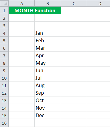
Now, you want to convert these names to the month in numbers.
You can use the following MONTH in Excel:
= MONTH ( DATEVALUE( B4 & ” 1”)


For Jan, the MONTH in Excel will return 1. For Feb, it will return 2 and so on.

MONTH in Excel Example #3
Suppose you have a list of holidays given in cells B3: B9 in a date-wise manner, as shown below.
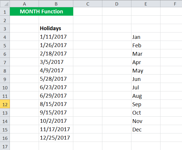
Now, you want to calculate the number of holidays each month. To do so, you can use the following MONTH formula in Excel for the first month given in E4:
= SUMPRODUCT( –( MONTH( $B$4:$B$16 ) = MONTH( DATEVALUE( E4 & ” 1″)) ) )

Then, drag it to the rest of the cells.
Let us look at the MONTH function in Excel detail:
- MONTH( $B$4:$B$16 ) will check the month of the dates provided in cell range B4:B16 in a number format. The MONTH function in Excel will return {1; 1; 2; 3; 4; 5; 6; 6; 8; 9; 10; 11; 12}
- MONTH( DATEVALUE( E4 & ” 1″) will give the month in number corresponding to cell E4 (see example 2). The MONTH function in Excel will return 1 for January
- SUMPRODUCT in ExcelThe SUMPRODUCT excel function multiplies the numbers of two or more arrays and sums up the resulting products.read more (– (…) = (..) ) will match the month given in B4:B16 with January (=1) and will add one each time when it is true.
Since January appears twice in the given data, the MONTH function in Excel will return 2.

Similarly, you can do for the rest of the cells.

MONTH in Excel Example #4
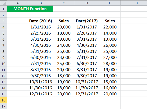
Suppose you have sales data for the past two years. The data was collected on the last date of the month. The data was manually entered, so there could be a mismatch in the data. You should compare the sales between 2016 and 2017 for each month.
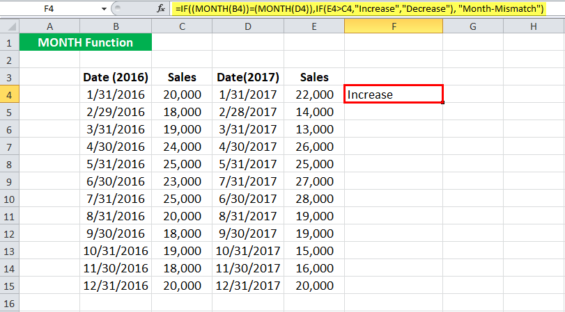
To check if the months are the same and then compare the sales, you can use the MONTH formula in Excel:
=IF( (MONTH(B4)) = (MONTH(D4) ), IF( E4 > C4, “Increase”, “Decrease” ), “Month-Mismatch” )

For the first entry, the MONTH function in Excel will return “Increase.”
Let us look at the MONTH in Excel in detail:
If the MONTH of B4 (for 2016) is equal to the MONTH given in D4 (for 2017),
- The MONTH function in Excel will check if the sales for the given month in 2017 are greater than that in 2016.
- If it is greater, it will return “Increase.”
- Else, it will return to “Decrease.”
If the MONTH of B4 (for 2016) is not equal to the MONTH given in D4 (for 2017),
- The MONTH function in Excel will return “Mismatch.”
Similarly, you can do for the rest of the cells.

You could also add another condition to check if the sales are equal and return “Constant.”
MONTH in Excel Example #5
Suppose you work in your company’s sales department and have date-wise data of how many products were sold on a particular date for the previous year, as shown below.

Now, you want to club the number of products monthly. To do so, you use the following MONTH formula in Excel:
= SUMPRODUCT(– ( EXACT( F4, MONTH( $B$4:$B$17 ))), $C$4:$C$17 )
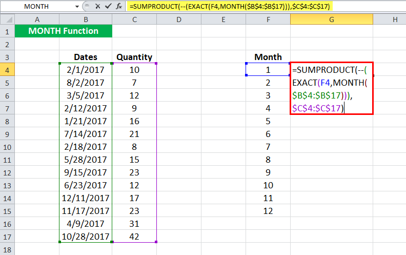
For the first cell, the MONTH function in Excel will return 16.

Then, drag it to the rest of the cells.

Let us look at the MONTH in Excel in detail:
= SUMPRODUCT(– ( EXACT( F4, MONTH( $B$4:$B$17 ))), $C$4:$C$17 )
- MONTH( $B$4:$B$17 ) will give the month of the cells in B4: B17. MONTH function in Excel will return a matrix {2; 8; 3; 2; 1; 7; 2; 5; 9; 6; 12; 11; 4; 10}
- EXACT( F4, MONTH( $B$4:$B$17 )) will match the month in F4 ( 1 here) with the matrix and will return another matrix with TRUE when it is a match or FALSE otherwise. For the 1st month, it will return {FALSE; FALSE; FALSE; FALSE; TRUE; FALSE; FALSE; FALSE; FALSE; FALSE; FALSE; FALSE; FALSE; FALSE}
- SUMPRODUCT (– (..), $C$4:$C$17) will sum the values in C4:C17 when the corresponding value in the matrix is “TRUE.”
The MONTH function in Excel will return 16 for January.

Things to remember about a MONTH in Excel
- The MONTH function returns the month of the given date or serial number.
- Excel MONTH function is given #VALUE! Error when it cannot recognize the date.
- The Excel MONTH function accepts dates only after 1 Jan 1900. It will provide the #VALUE! Error when the input date is earlier than 1 Jan 1900.
- The MONTH function in Excel returns the month in number format only. Therefore, its output is always a number between 1 and 12.
MONTH Excel Function Video
Recommended Articles
This article is a guide to MONTH Function in Excel. We discuss the MONTH formula in Excel and how to use the MONTH function, along with Excel examples and downloadable Excel templates. You may also look at these useful functions in Excel: –
- EDATE Function in ExcelEDATE is a date and time function in excel which adds a given number of months into a date and gives us a date in a numerical format of date. It takes dates and integers as input, the output returned by this function is also a date value. read more
- VBA MONTH VBA Month Function is an inbuilt function that is used to extract the month from a date. The output of this function is an integer ranging from 1 to 12. Only the month number is extracted from the supplied date value by this function.read more
- EOMONTH in ExcelEOMONTH is a worksheet date function in excel which calculates the end of the month for the given date by adding a specified number of months to the arguments. This function takes two arguments: the date and another as integer, and the output is in the date format.read more
- FREQUENCY Excel FunctionThe FREQUENCY function in Excel calculates the number of times a data values occurs within a given range of values and returns a vertical array of numbers corresponding to each value’s frequency within a range.read more
Excel for Microsoft 365 Excel for Microsoft 365 for Mac Excel for the web Excel 2021 Excel 2021 for Mac Excel 2019 Excel 2019 for Mac Excel 2016 Excel 2016 for Mac Excel 2013 Excel 2010 Excel 2007 Excel for Mac 2011 Excel Starter 2010 More…Less
This article describes the formula syntax and usage of the MONTH function in Microsoft Excel.
Description
Returns the month of a date represented by a serial number. The month is given as an integer, ranging from 1 (January) to 12 (December).
Syntax
MONTH(serial_number)
The MONTH function syntax has the following arguments:
-
Serial_number Required. The date of the month you are trying to find. Dates should be entered by using the DATE function, or as results of other formulas or functions. For example, use DATE(2008,5,23) for the 23rd day of May, 2008. Problems can occur if dates are entered as text.
Remarks
Microsoft Excel stores dates as sequential serial numbers so they can be used in calculations. By default, January 1, 1900 is serial number 1, and January 1, 2008 is serial number 39448 because it is 39,448 days after January 1, 1900.
Values returned by the YEAR, MONTH and DAY functions will be Gregorian values regardless of the display format for the supplied date value. For example, if the display format of the supplied date is Hijri, the returned values for the YEAR, MONTH and DAY functions will be values associated with the equivalent Gregorian date.
Example
Copy the example data in the following table, and paste it in cell A1 of a new Excel worksheet. For formulas to show results, select them, press F2, and then press Enter. If you need to, you can adjust the column widths to see all the data.
|
Date |
||
|---|---|---|
|
15-Apr-11 |
||
|
Formula |
Description |
Result |
|
=MONTH(A2) |
Month of the date in cell A2 |
4 |
See Also
DATE function
Add or subtract dates
Date and time functions (reference)
Need more help?
Note: This example assumes the start date will be provided as the first of the month. See below for a formula that will automatically return the first day of the current month.
In this example, the goal is to generate a dynamic calendar for any given month, based on a start date entered in cell J6, which is named «start» We assume that start is a valid first-of-month date like 1-Jan-2022, 1-Feb-2022, 1-Mar-2022, etc. The final calendar should place each day of the month in a grid with each week starting on Sunday, as seen in the example. The solution explained below is based on the SEQUENCE function. SEQUENCE is one of the original dynamic array functions in Excel, and a perfect fit for this problem.
Background study
- Dynamic array formulas in Excel — overview
- The SEQUENCE function — 3 min video
- WEEKDAY function — overview and examples
- Custom number formats in Excel — overview
Short version
The explanation below is rather long. The short version is that the SEQUENCE function outputs a 6 x 7 array of 42 dates in a calendar grid, formatted to display the day only. This works, because Excel dates are just serial numbers. The main challenge with this problem is figuring out what date to start with for a given month, which is always a Sunday. This is handled with the CHOOSE and WEEKDAY functions. Conditional formatting is used to highlight the current date and holidays, and lighten days in other months. Read below for all the details.
Basic SEQUENCE
The SEQUENCE function can be used to generate numeric sequences. For example, to generate the numbers 1 to 10 in ten rows, you can use SEQUENCE like this:
=SEQUENCE(10) // returns {1;2;3;4;5;6;7;8;9;10}
The result is an array that contains the numbers 1-10. The array spills into a vertical range of ten cells. SEQUENCE can generate arrays in rows and columns. For example, the following formula creates the numbers 1-10 in an array with 5 rows and 2 columns:
=SEQUENCE(5,2)
And the formula below will fill a 7 x 6 grid of cells with the numbers 1-42:
=SEQUENCE(6,7)
The screen below shows how these formulas behave on a worksheet:

These are just numbers, not dates, but you can see the core concept.
SEQUENCE with dates
Because Excel dates are just large serial numbers, the SEQUENCE function can easily be used to generate arrays of dates. For example, the formula below will generate dates for the 31 days of January 2022:
=SEQUENCE(7,1,DATE(2022,1,1))
Note: the DATE function is a safer way to hard code dates into formulas, since dates entered as text can be misinterpreted.
To translate: we are asking for 7 numbers, in a 7 x 1 array, starting with January 1, 2022. SEQUENCE automatically defaults to a step value of 1, so the result is a list of serial numbers starting with 44562. Obviously, we don’t want to display serial numbers in our calendar, we want to show days. To do that we can use the custom number format «d». That will cause Excel to display just the day numbers. The screen below shows before and after:

Now let’s see what happens if we ask for 6 x 7 grid, starting with January 1, 2022:
=SEQUENCE(6,7,DATE(2022,1,1))
Once we format the output with the custom number format «d», we see a total of 42 numbers, beginning with January 1. At the end of January, the month changes to February and the day becomes 1 again:

We still don’t have a usable calendar, but we’re getting closer!
To make a proper calendar, we need the first day in our grid to start on Sunday. If the first day of a month is not a Sunday, we need to start the grid on the last Sunday of the previous month. How can we calculate the last Sunday of the previous month? Before we get into specific functions, let’s clarify the goal.
First Sunday
If the first of a month happens to be a Sunday, we’re done. There’s no need to do anything. The first of the month is our start date. However, if the first of the month is not a Sunday, we need to «roll back» some number of days to the prior Sunday. How many days do we need to roll back? This depends on what day of the week the first day of a month lands on. For example, if the first is a Tuesday, we need to roll back 2 days. If the first is a Friday, we need to roll back 5 days. And if the first is already a Sunday, we need to roll back 0 days.
Now we have a pretty good idea of what we need to do, we just need to implement that behavior in a formula. This is where the formula gets a bit tricky, because we need to combine two functions, WEEKDAY and CHOOSE, in a way that most users won’t recognize.
The WEEKDAY function
To figure out the day of week, we use the WEEKDAY function. WEEKDAY returns a number for each day of the week. By default, WEEKDAY returns 1 for Sunday and 7 for Saturday. For example, WEEKDAY returns 7 for January 1, 2022, since the first is a Saturday:
=WEEKDAY(DATE(2022,1,1)) // returns 7
For January 2, 2022, WEEKDAY returns 1, since the second is a Sunday:
=WEEKDAY(DATE(2022,1,2)) // returns 1
To summarize, WEEKDAY will give us a number between 1-7 for each day of the week, and we can use that result to figure out how many days we need to roll back.
The CHOOSE function
The CHOOSE function is used to select arbitrary values by numeric position. For example, if we have the colors «red», «blue», and «green», we can use CHOOSE like this:
=CHOOSE(1,"red", "blue", "green") // returns "red"
=CHOOSE(2,"red", "blue", "green") // returns "blue"
=CHOOSE(3,"red", "blue", "green") // returns "green"
CHOOSE is a flexible function and accepts a list of text values, numbers, cell references, in any combination.
CHOOSE + WEEKDAY
Next, we’re going to combine CHOOSE and WEEKDAY to give us the correct «roll back» number like this:
=CHOOSE(WEEKDAY(start),0,1,2,3,4,5,6)
The index_num argument is provided by the WEEKDAY function. The other individual values given to CHOOSE are the roll back numbers, one for each day of the week. WEEKDAY returns a number between 1-7, and the CHOOSE function uses the number from WEEKDAY to select a number from the list of numbers provided. For example, if WEEKDAY returns 3 (Tuesday), CHOOSE returns 2:
CHOOSE(3,0,1,2,3,4,5,6) // returns 2
Now we are finally ready to use this roll back number to compute the first Sunday in the grid. Because dates are just numbers in Excel, the operation is simple – we just need to subtract the roll back number from the start date:
start-CHOOSE(WEEKDAY(start),0,1,2,3,4,5,6) // first Sunday
The result is a valid date that represents the first Sunday in the calendar grid.
Putting it all together
Now we need to combine the ideas explained above into a single formula based on the SEQUENCE function. We start off by asking for a 6 x 7 array of numbers like this:
=SEQUENCE(6,7 // 6 rows, 7 columns
Then, for the start argument, we simply provide the code we worked out above:
=SEQUENCE(6,7,start-CHOOSE(WEEKDAY(start),0,1,2,3,4,5,6))
The result is a full grid of 42 dates that can be displayed as a monthly calendar. If the start date in J6 is changed to another first of month date, the grid automatically updates.
Conditional formatting rules
The conditional formatting rules to highlight the current date and holidays, and lighten days in other months are listed below:

The formula for the current date is:
=B6=TODAY()
The formula to highlight holidays is based on the COUNTIF function:
=COUNTIF(holidays,B6)
If the count is anything but zero, the date must be a holiday. Holidays must be a range that contains valid Excel dates that represent non-working days. In the example shown, holidays is the named range L6:L8. You can add more holidays to this list as you like, but don’t forget to update the named range. Alternatively, you can define holidays as an Excel Table so the range updates automatically.
The formula to lighten days in other months is based on the MONTH function:
=MONTH(B6)<>MONTH(start)
If the month of the current date is different from the month of the date in J6, trigger the rule.
Read more: Conditional formatting with formulas, Excel custom number formats
Calendar title
The formula to output the calendar title in cell B4 is based on the TEXT function:
=TEXT(start,"mmmm yyyyy")
The title is centered over the calendar grid with the Center Across Selection. Select B4:H4, and use Control + 1 to open Format Cells, then select «Center Across Selection» from the Horizontal text alignment dropdown. This is a better option than merge cells, since it doesn’t alter the grid structure in the worksheet.
Perpetual calendar with current date
To create a perpetual calendar that updates automatically based on the current date, we need to update the formula to generate the first day of the current month on the fly. The first day of the current month can be calculated with the EOMONTH function like this:
=EOMONTH(TODAY(),-1)+1
You can use this formula directly in cell J6 and the calendar will always stay up to date. For an all-in-one formula, we can add the LET function like this:
=LET(start,EOMONTH(TODAY(),-1)+1,SEQUENCE(6,7,start-CHOOSE(WEEKDAY(start),0,1,2,3,4,5,6)))
Here, we use the LET function to define «start» as the first day of the current month, then run the original formula unchanged. The local variable «start» overrides the named range start on the worksheet, which can be deleted if desired.
Monday start
To generate a calendar that starts on Monday instead of Sunday, you can use the following code inside of SEQUENCE as the start argument:
=start-CHOOSE(WEEKDAY(start),6,0,1,2,3,4,5)
Using the same logic explained above, this code rolls back the start date as needed to begin the calendar on Monday. This example has more information on rolling back dates to previous days of the week.
Excel spreadsheets provide the ability to work with various types of textual and numerical information. Date processing is also available. In this case, there may be a need to extract from the general meaning of a specific number, for example, a year. There are separate functions for this: YEAR, MONTH, DAY and DAY.
Examples of using functions for date processing in Excel
Excel tables store dates that are presented as a sequence of numeric values. It begins on January 1, 1900. This date will correspond to the number 1. At the same time, January 1, 2009 is laid down in the tables, as the number 39813. This is the number of days between the two designated dates.
The function YEAR is used similarly to the adjacent:
- MONTH;
- DAY;
- WEEKDAY.
All of them display numerical values corresponding to the Gregorian calendar. Even if in the Excel spreadsheet, the Hijra calendar was chosen to display the entered date, then when isolating the year and other composite values by functions, the application will present a number that is equivalent to the Gregorian system of chronology.
To use the YEAR function, you need to enter into the cell the following function formula with one argument:
=YEAR(cell address with date in numeric format)
The function argument is required. It can be replaced by «date_number_number». In the examples below, you can clearly see this. It is important to remember that when displaying the date as text (automatic orientation on the left edge of the cell), the YEAR function will not be executed. Its result will be the # SIGN. Therefore, formatted dates must be presented in a numerical version. Days, months and year can be separated by a dot, slash or comma.
Consider an example of working with the YEAR function in Excel. If we need to get a year from the original date, the function AVAILABLE will not help us since it does not work with dates, but only with text and numeric values. To separate the year, month or day from the full date for this, Excel provides functions for working with dates.
Example: There is a table with a list of dates and in each of them it is necessary to separate the value of only the year.
We introduce the original data in Excel.
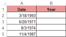
To solve the problem, it is necessary to enter the formula in the cells of column B:
=YEAR(the address of the cell, from the date of which you need to isolate the year value)
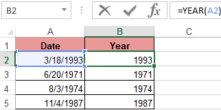
As a result, we extract years from each date.
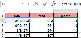
A similar example of the MONTH function in Excel:
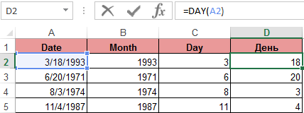
An example of working with functions DAY and WEEKDAY. The DAY function gets to calculate from the date the number of any day:
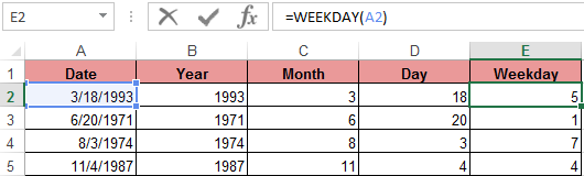
WEEKDAY function returns the number of the day of the week (1-Monday, 2-Tuesday …, etc.) for any date:
In the second optional argument of the WEEKDAY function, the number 2 may specified for our day of the week countdown format (Monday-1 through Sunday-7):
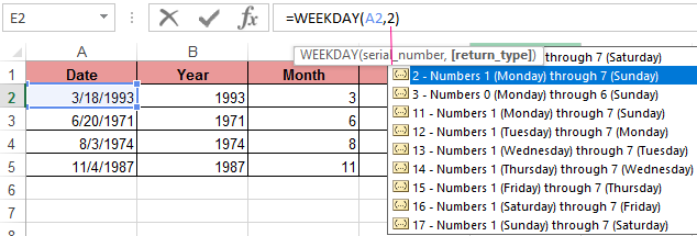
If you omit the second optional argument, then the default format will be used (English from Sunday-1 to Saturday-7).
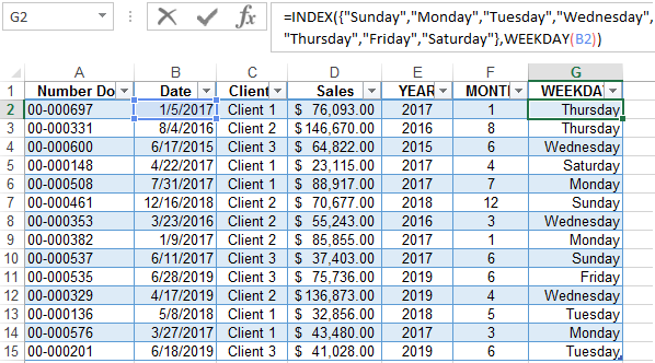
Create a formula of the combination of the functions INDEX and WEEKDAY:
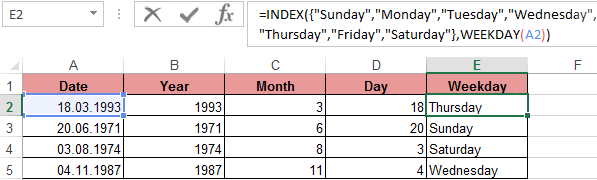
We obtain a more understandable form of the implementation of this function.
Examples of the practical use of functions for working with dates
These primitive functions are very useful when grouping data by: years, months, days of the week, and specific days.
Suppose we have a simple sales report:
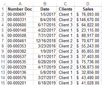
We need to quickly organize data for visual analysis without using pivot tables. To do this, we will bring the report into a table where it is convenient and quickly to group data by year, month and day of the week:
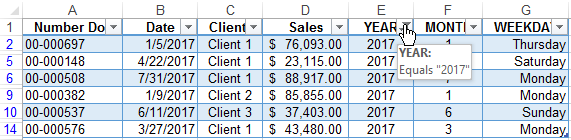
Now we have a tool to work with this sales report. We can filter and segment data by specific time criteria:
In addition, you can make a histogram to analyze the best-selling days of the week, to understand which day of the week has the largest number of sales:
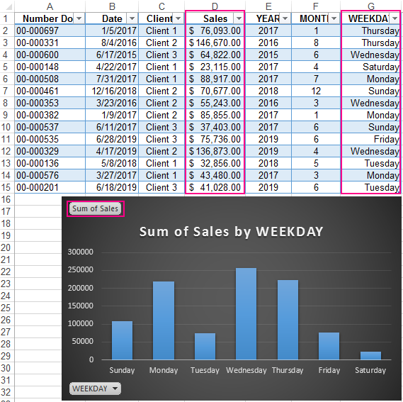
In this form, it is very convenient to segment sales reports for long, medium and short periods of time.
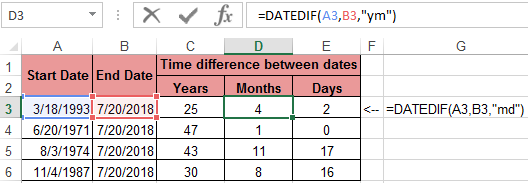
It should be immediately noted that in order to get the difference between the two dates, none of the above functions will help us. For this task, you should use a specially designed function DATEDIF:
Download examples fo functions YEAR MONTH DAY WEEKDAY and DATEDIF
The type of values in the date cells requires a special approach to data processing. Therefore, you should use the appropriate type of function in Excel.
In this post, we can learn how to easily create a monthly calendar in Excel 365 using some of the date functions and the Sequence.
It’s a dynamic monthly calendar that updates when you change month and year. In addition to that, there are rooms given for entering notes below dates. The formula won’t break.
Because of the dynamic array feature in Excel 365, some of the formulas SPILL their results. The Sequence is one such function.
Actually, a single piece of code (a formula in one cell) in Excel 365 can populate a whole month’s calendar. But the problem with such a formula is it would break when you hand enter any texts (notes) below the dates.
So I have broken the formula into six pieces and entered them in the very first cell of every alternate row. This way, I could give room for entering notes without breaking the formula.
Let’s see how to easily create a dynamic monthly calendar in Excel 365 using formulas.
To make the calendar dynamic (supports user interaction), we should provide two cells to input the month and year. So when changing those values, the calendar will update.
In the following example, cells G1 and H1 are those input cells.

Prerequisites
To avoid typos, you may create a drop-down in cell G1 with the month names to select.
To do that in Excel 365, you can follow the below few steps.
1. Make sure that the active cell is G1.
2. Under the “Data” menu, find the “Data Validation” under the “Data Tools.” Click it.
3. Select “List.”
4. Paste the text January, February, March, April, May, June, July, August, September, October, November, December within the “Source” field.
5. Click OK.

Now one more thing to do. In cell range B3:H3, enter the day names from Sunday to Monday.
Formula to Create a Dynamic Monthly Calendar in Excel 365
Insert the below formula in cell B5 (You won’t get the correct result. I’ll come to that.)
=SEQUENCE(1,7,DATE(H1,MONTH(G1&1),1)-WEEKDAY(DATE(H1,MONTH(G1&1),1))+1)Before moving to the next step, let’s learn this Excel 365 formula.
How Does this Formula Spill Dates?
The above Excel formula returns dates or date values in one row and seven columns as per the syntax SEQUENCE(ROWS, COLUMNS, START)
The start value within the Sequence determines the date to start. Here is that formula.
=DATE(H1,MONTH(G1&1),1)-WEEKDAY(DATE(H1,MONTH(G1&1),1))+1Let’s split this Excel 365 formula into two parts.
Part_1
=DATE(H1,MONTH(G1&1),1)It returns the first day of the month of the selected month in cell G1.
Part_2
=WEEKDAY(DATE(H1,MONTH(G1&1),1))It returns the weekday number of the above part_1 date. So part_1 - part_2+1 will be the week start date (Sunday).
Supporting Formulas
Insert the following formulas in cells B7, B9, B11, B13, and B15.
B7
=SEQUENCE(1,7,H5+1)B9
=SEQUENCE(1,7,H7+1)B11
=SEQUENCE(1,7,H9+1)B13
=SEQUENCE(1,7,H11+1)B15
=SEQUENCE(1,7,H13+1)The result of the above Excel 365 formulas may be date values. So select those dates (rows 5, 7, 9, 11, 13, and 15) and format them to date.
To do that, under the “Format” menu, find the “Cells” group. Within that group, click Format -> Format Cells. Alternatively, you can use the shortcut Ctrl+1.
Under the “Number” tab, select “Date” and choose the format that you wish to apply.
We require to follow one more step to finishing our custom Monthly Calendar Using Formulas in Excel 365. That’s conditional formatting.
Hide Certain Dates By Changing Font Color
We have created a monthly calendar in Excel 365 using a limited number of formulas. But there is one unaddressed issue.
You can see some of the dates that fall in the previous/next months of the selected month in cell G1.

Follow the below steps to hide those dates. That’s the final step to create a dynamic calendar in Excel 365.
Steps
1. Select B5:H15.
2. Click “Conditional Formatting” under the “Home” tab “Styles” group.
3. Click “New Rule”.
4. Under “Select a Rule Type,” choose “Use a formula to determine which cells to format.”

5. Insert the below formula in the field provided.
=MONTH(B5)<>MONTH($G$1&1)6. Click “Format” and choose “Font” color to White.
7. Click OK -> OK and voila!
This way, we can create a dynamic monthly calendar in Excel 365.