Formula for the date in excel

To get detailed information about a function, click its name in the first column.

Note: Version markers indicate the version of Excel a function was introduced. These functions aren’t available in earlier versions. For example, a version marker of 2013 indicates that this function is available in Excel 2013 and all later versions.

Function	Description
DATE function	Returns the serial number of a particular date
DATEDIF function	Calculates the number of days, months, or years between two dates. This function is useful in formulas where you need to calculate an age.
DATEVALUE function	Converts a date in the form of text to a serial number
DAY function	Converts a serial number to a day of the month
DAYS function	Returns the number of days between two dates
DAYS360 function	Calculates the number of days between two dates based on a 360-day year
EDATE function	Returns the serial number of the date that is the indicated number of months before or after the start date
EOMONTH function	Returns the serial number of the last day of the month before or after a specified number of months
HOUR function	Converts a serial number to an hour
ISOWEEKNUM function	Returns the number of the ISO week number of the year for a given date
MINUTE function	Converts a serial number to a minute
MONTH function	Converts a serial number to a month
NETWORKDAYS function	Returns the number of whole workdays between two dates
NETWORKDAYS.INTL function	Returns the number of whole workdays between two dates using parameters to indicate which and how many days are weekend days
NOW function	Returns the serial number of the current date and time
SECOND function	Converts a serial number to a second
TIME function	Returns the serial number of a particular time
TIMEVALUE function	Converts a time in the form of text to a serial number
TODAY function	Returns the serial number of today’s date
WEEKDAY function	Converts a serial number to a day of the week
WEEKNUM function	Converts a serial number to a number representing where the week falls numerically with a year
WORKDAY function	Returns the serial number of the date before or after a specified number of workdays
WORKDAY.INTL function	Returns the serial number of the date before or after a specified number of workdays using parameters to indicate which and how many days are weekend days
YEAR function	Converts a serial number to a year
YEARFRAC function	Returns the year fraction representing the number of whole days between start_date and end_date

Important: The calculated results of formulas and some Excel worksheet functions may differ slightly between a Windows PC using x86 or x86-64 architecture and a Windows RT PC using ARM architecture. Learn more about the differences.

For work with dates in Excel, in the category «Date and time» is defined in the functions section. Let`s consider the most prevalent functions in this category.



How Excel Processes Time

The Excel program «perceives» the date and time as an ordinary number. The spreadsheet converts to such number, equating the day to unity. As a result, the time value represents a fraction of unity. For example, 12. 00 — is 0. 5.

The date value to the spreadsheet converts to a number which equal to the number of days from January 1, 1900 (so the developers decided) to the specified date. For example, when converting the date 13. 04. 1987, the number is 31880. That is, from 1. 01. 1900 passed 31. 880 days.

This principle underlies in the basis of the calculations of the time data. To find the number of days between two dates, it`s enough to take an earlier period from a later time one.



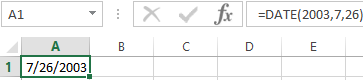
The example of DATE function

You need to describe of the date value with compiling it with individual elements of numbers.

There is the syntax: year; month, day.

All arguments are required. They can be specified by numbers or by reference to cells with the corresponding numeric data: for the year — from 1900 to 9999; for the month — from 1 to 12; for the day — from 1 to 31.

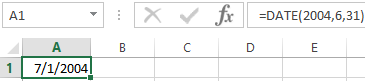
If you point a larger number for the «Day» argument (than the number of days in the pointed month), you receive the extra days, will be passed to the next month. For example, specifying 32 days for December, we will receive as a result on January 1.

The example of using the function:

Let’s set more days for June:

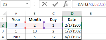
Examples of using the cell references as arguments:

The DATEDIF function in Excel

It returns the difference between two dates.

The arguments:

• start date;
• final date;
• the code indicating to the units of counting (days, months, years, etc.).

The methods of measuring intervals between the given dates:

• to display the result in days — «d»;
• in months – «m»;
• in years – «y»;
• in months without years – «ym»;
• in days without months and years – «md»;
• in days without years – «yd».

In some versions of Excel, if you use the last two arguments («md», «yd»), the function may give an error. It is better to use to alternative formulas.

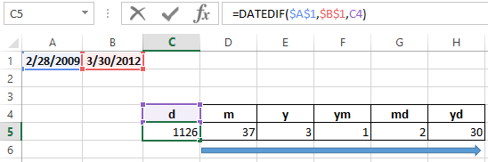
The examples of the operation the DATEDIF function:

In Excel 2007 version, this function is not in the directory, but it works. But you need to check the results are better, because there are flaws possible.

The YEAR function in Excel

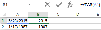
It returns the year as an integer number (from 1900 to 9999), what corresponds to the specified date. There is only one argument must be entered in the structure of the function – is the date in a numerical format. The argument must be entered using the DATE function or represents to the result of evaluating other formulas.

The example of using the YEAR function:

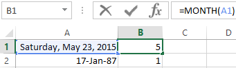
The MONTH function in Excel: the example

It returns the month as an integer number (from 1 to 12) for a date is specified in a numeric format. The argument – is the date of the month that you want to show in a numerical format. The dates in the text format this function does not handle correctly.

The examples of using the MONTH function:

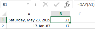
The examples of DAY, WEEKDAY and functions WEEKNUM in Excel

It returns the day as an integer number (from 1 to 31) for a date specified in a numeric format. The argument – it is the date of the day you want to find in a numerical format.

For returning of the weekday ordinal of the specified date, you can apply the function WEEKDAY:

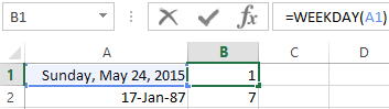
By default, the function considers Sunday the 1-st day of the week.

To display of the ordinal number of the week for the pointed date, you should use the WEEKNUM function:

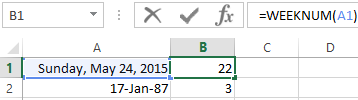
The date of 24. 05. 2015 is 22 week in a year. The week starts on Sunday (by default).

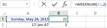
As the second argument the figure 2 is specified. Therefore, the formula considers that the week starts on Monday (the 2-d day of the week).

Download all examples functions for working with dates

For indicating of the current date, the function TODAY (no arguments) is used. To display the current time and date, the function NOW() is used.

Одной из самых востребованных групп операторов при работе с таблицами Excel являются функции даты и времени. Именно с их помощью можно проводить различные манипуляции с временными данными. Дата и время зачастую проставляется при оформлении различных журналов событий в Экселе. Проводить обработку таких данных – это главная задача вышеуказанных операторов. Давайте разберемся, где можно найти эту группу функций в интерфейсе программы, и как работать с самыми востребованными формулами данного блока.

Работа с функциями даты и времени

Группа функций даты и времени отвечает за обработку данных, представленных в формате даты или времени. В настоящее время в Excel насчитывается более 20 операторов, которые входят в данный блок формул. С выходом новых версий Excel их численность постоянно увеличивается.

Любую функцию можно ввести вручную, если знать её синтаксис, но для большинства пользователей, особенно неопытных или с уровнем знаний не выше среднего, намного проще вводить команды через графическую оболочку, представленную Мастером функций с последующим перемещением в окно аргументов.

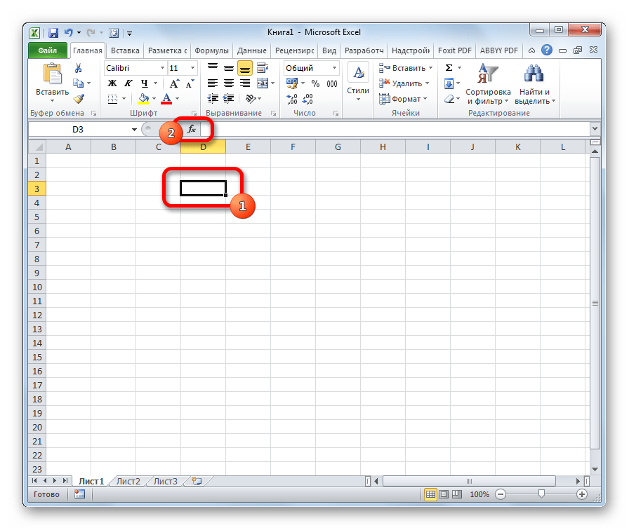
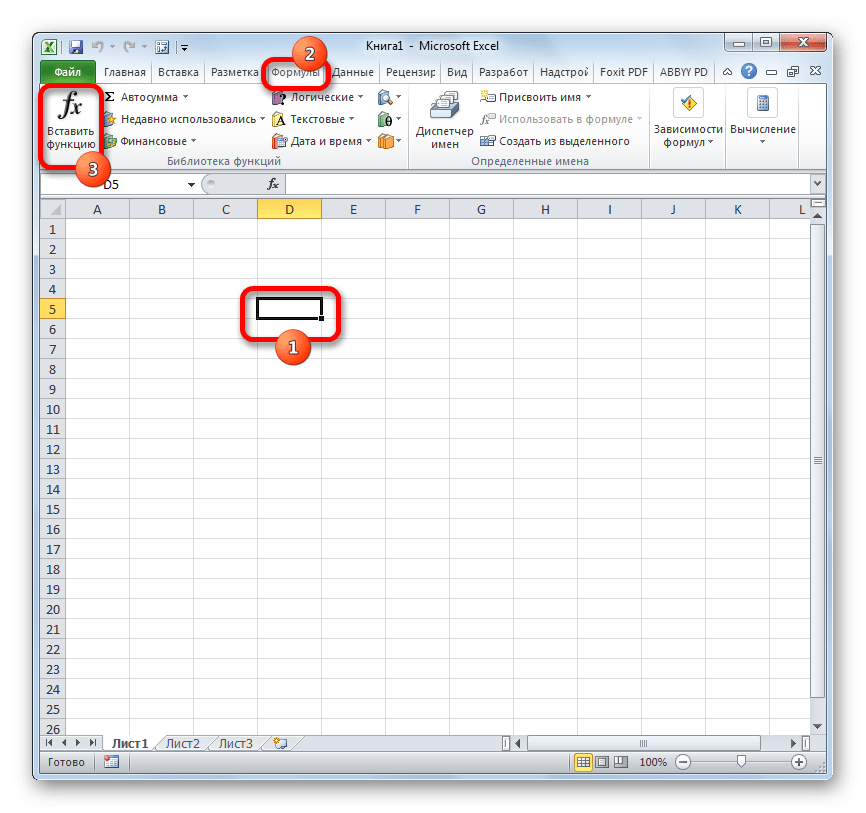
1. Для введения формулы через Мастер функций выделите ячейку, где будет выводиться результат, а затем сделайте щелчок по кнопке «Вставить функцию». Расположена она слева от строки формул.



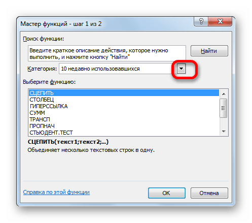
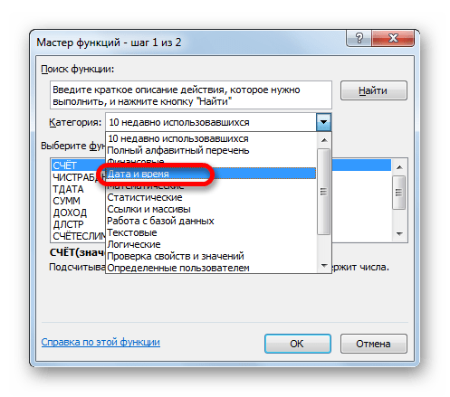
2. После этого происходит активация Мастера функций. Делаем клик по полю «Категория».



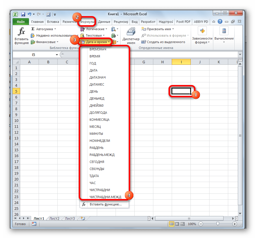
3. Из открывшегося списка выбираем пункт «Дата и время».



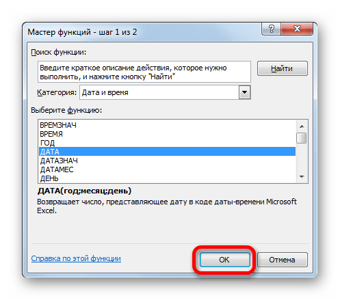
4. После этого открывается перечень операторов данной группы. Чтобы перейти к конкретному из них, выделяем нужную функцию в списке и жмем на кнопку «OK». После выполнения перечисленных действий будет запущено окно аргументов.

Кроме того, Мастер функций можно активировать, выделив ячейку на листе и нажав комбинацию клавиш Shift+F3. Существует ещё возможность перехода во вкладку «Формулы», где на ленте в группе настроек инструментов «Библиотека функций» следует щелкнуть по кнопке «Вставить функцию».

Имеется возможность перемещения к окну аргументов конкретной формулы из группы «Дата и время» без активации главного окна Мастера функций. Для этого выполняем перемещение во вкладку «Формулы». Щёлкаем по кнопке «Дата и время». Она размещена на ленте в группе инструментов «Библиотека функций». Активируется список доступных операторов в данной категории. Выбираем тот, который нужен для выполнения поставленной задачи. После этого происходит перемещение в окно аргументов.

Урок: Мастер функций в Excel

ДАТА

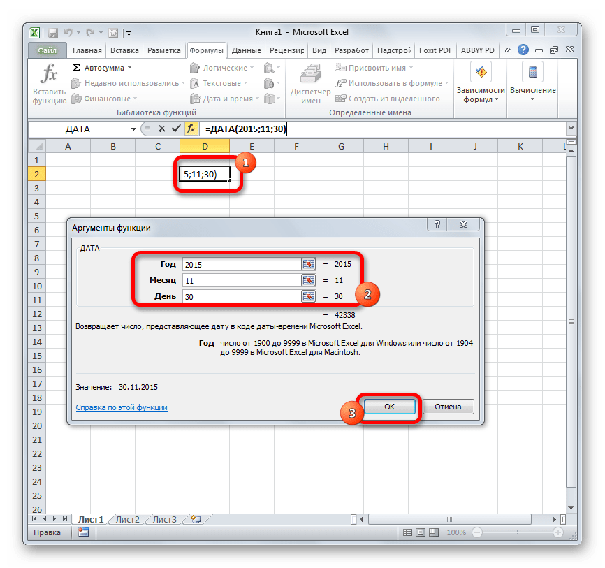
Одной из самых простых, но вместе с тем востребованных функций данной группы является оператор ДАТА. Он выводит заданную дату в числовом виде в ячейку, где размещается сама формула.

Его аргументами являются «Год», «Месяц» и «День». Особенностью обработки данных является то, что функция работает только с временным отрезком не ранее 1900 года. Поэтому, если в качестве аргумента в поле «Год» задать, например, 1898 год, то оператор выведет в ячейку некорректное значение. Естественно, что в качестве аргументов «Месяц» и «День» выступают числа соответственно от 1 до 12 и от 1 до 31. В качестве аргументов могут выступать и ссылки на ячейки, где содержатся соответствующие данные.

Для ручного ввода формулы используется следующий синтаксис:

=ДАТА(Год;Месяц;День)

Близки к этой функции по значению операторы ГОД, МЕСЯЦ и ДЕНЬ. Они выводят в ячейку значение соответствующее своему названию и имеют единственный одноименный аргумент.

РАЗНДАТ

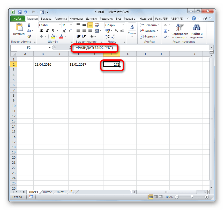
Своего рода уникальной функцией является оператор РАЗНДАТ. Он вычисляет разность между двумя датами. Его особенность состоит в том, что этого оператора нет в перечне формул Мастера функций, а значит, его значения всегда приходится вводить не через графический интерфейс, а вручную, придерживаясь следующего синтаксиса:

=РАЗНДАТ(нач_дата;кон_дата;единица)

Из контекста понятно, что в качестве аргументов «Начальная дата» и «Конечная дата» выступают даты, разницу между которыми нужно вычислить. А вот в качестве аргумента «Единица» выступает конкретная единица измерения этой разности:

• Год (y);
• Месяц (m);
• День (d);
• Разница в месяцах (YM);
• Разница в днях без учета годов (YD);
• Разница в днях без учета месяцев и годов (MD).

Урок: Количество дней между датами в Excel

ЧИСТРАБДНИ

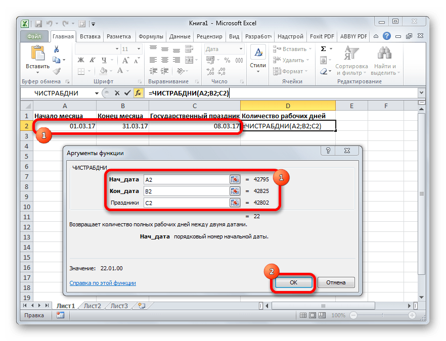
В отличии от предыдущего оператора, формула ЧИСТРАБДНИ представлена в списке Мастера функций. Её задачей является подсчет количества рабочих дней между двумя датами, которые заданы как аргументы. Кроме того, имеется ещё один аргумент – «Праздники». Этот аргумент является необязательным. Он указывает количество праздничных дней за исследуемый период. Эти дни также вычитаются из общего расчета. Формула рассчитывает количество всех дней между двумя датами, кроме субботы, воскресенья и тех дней, которые указаны пользователем как праздничные. В качестве аргументов могут выступать, как непосредственно даты, так и ссылки на ячейки, в которых они содержатся.

Синтаксис выглядит таким образом:

=ЧИСТРАБДНИ(нач_дата;кон_дата;[праздники])

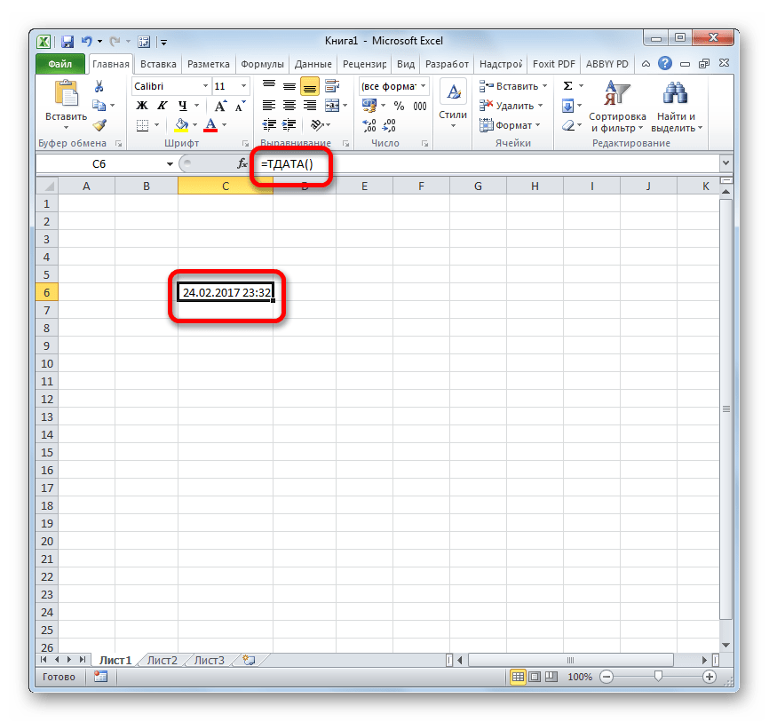
ТДАТА

Оператор ТДАТА интересен тем, что не имеет аргументов. Он в ячейку выводит текущую дату и время, установленные на компьютере. Нужно отметить, что это значение не будет обновляться автоматически. Оно останется фиксированным на момент создания функции до момента её перерасчета. Для перерасчета достаточно выделить ячейку, содержащую функцию, установить курсор в строке формул и кликнуть по кнопке Enter на клавиатуре. Кроме того, периодический пересчет документа можно включить в его настройках. Синтаксис ТДАТА такой:

=ТДАТА()

СЕГОДНЯ

Очень похож на предыдущую функцию по своим возможностям оператор СЕГОДНЯ. Он также не имеет аргументов. Но в ячейку выводит не снимок даты и времени, а только одну текущую дату. Синтаксис тоже очень простой:

=СЕГОДНЯ()

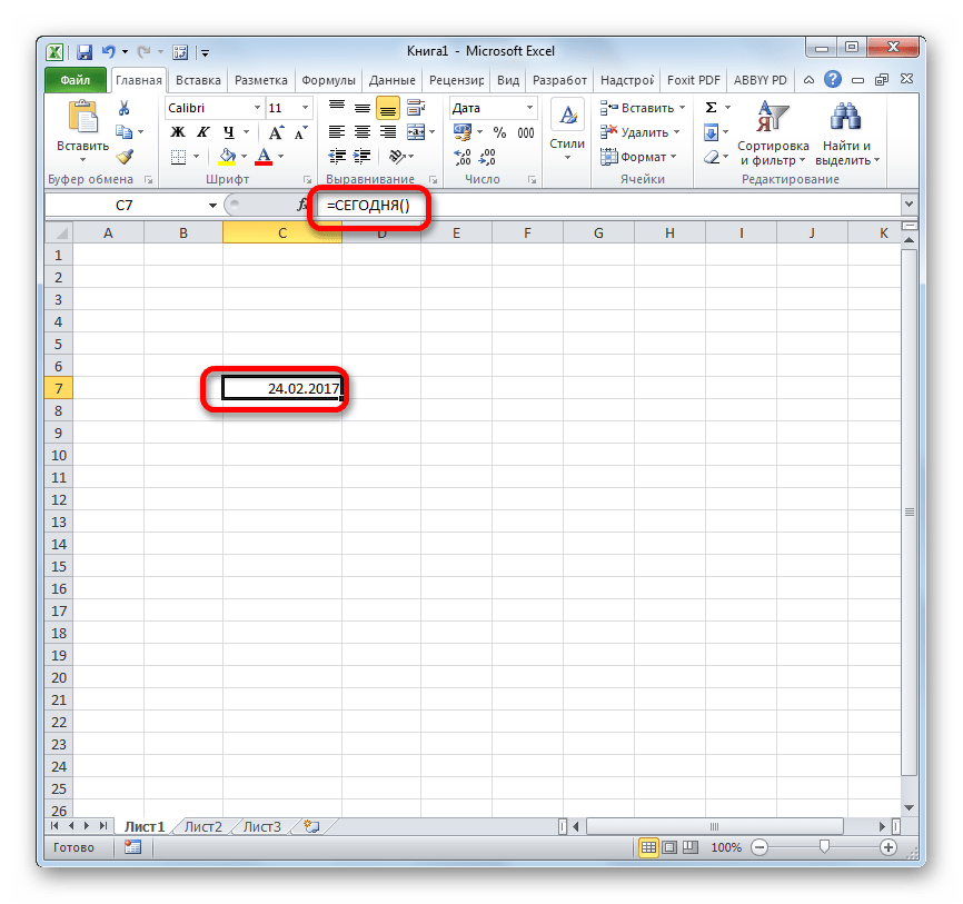
Эта функция, так же, как и предыдущая, для актуализации требует пересчета. Перерасчет выполняется точно таким же образом.

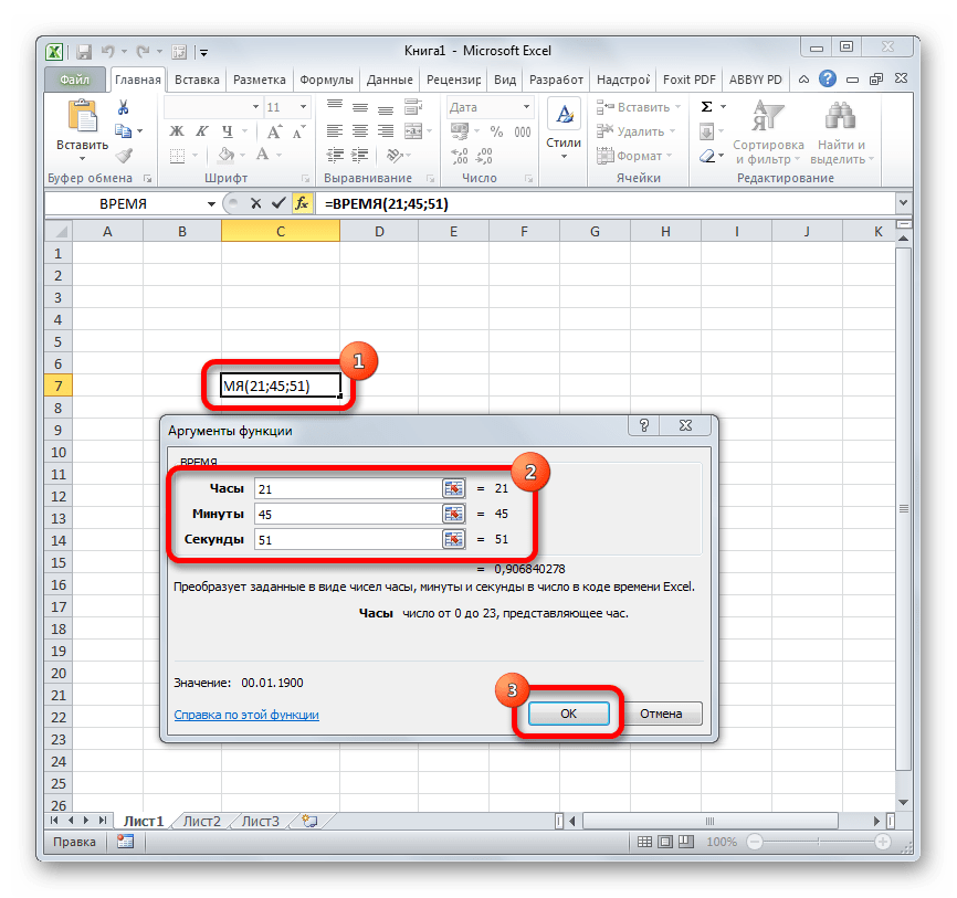
ВРЕМЯ

Основной задачей функции ВРЕМЯ является вывод в заданную ячейку указанного посредством аргументов времени. Аргументами этой функции являются часы, минуты и секунды. Они могут быть заданы, как в виде числовых значений, так и в виде ссылок, указывающих на ячейки, в которых хранятся эти значения. Эта функция очень похожа на оператор ДАТА, только в отличии от него выводит заданные показатели времени. Величина аргумента «Часы» может задаваться в диапазоне от 0 до 23, а аргументов минуты и секунды – от 0 до 59. Синтаксис такой:

=ВРЕМЯ(Часы;Минуты;Секунды)

Кроме того, близкими к этому оператору можно назвать отдельные функции ЧАС, МИНУТЫ и СЕКУНДЫ. Они выводят на экран величину соответствующего названию показателя времени, который задается единственным одноименным аргументом.

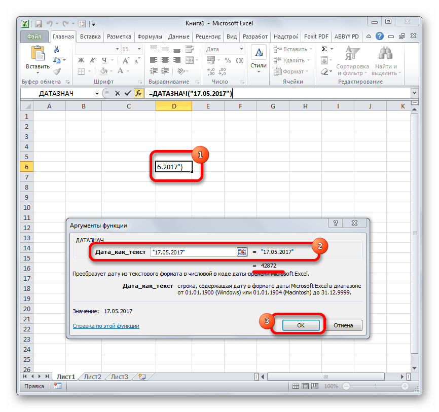
ДАТАЗНАЧ

Функция ДАТАЗНАЧ очень специфическая. Она предназначена не для людей, а для программы. Её задачей является преобразование записи даты в обычном виде в единое числовое выражение, доступное для вычислений в Excel. Единственным аргументом данной функции выступает дата как текст. Причем, как и в случае с аргументом ДАТА, корректно обрабатываются только значения после 1900 года. Синтаксис имеет такой вид:

=ДАТАЗНАЧ (дата_как_текст)

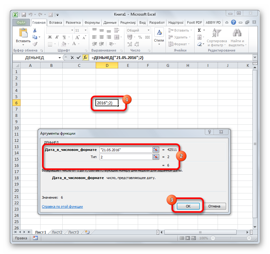
ДЕНЬНЕД

Задача оператора ДЕНЬНЕД – выводить в указанную ячейку значение дня недели для заданной даты. Но формула выводит не текстовое название дня, а его порядковый номер. Причем точка отсчета первого дня недели задается в поле «Тип». Так, если задать в этом поле значение «1», то первым днем недели будет считаться воскресенье, если «2» — понедельник и т.д. Но это не обязательный аргумент, в случае, если поле не заполнено, то считается, что отсчет идет от воскресенья. Вторым аргументом является собственно дата в числовом формате, порядковый номер дня которой нужно установить. Синтаксис выглядит так:

=ДЕНЬНЕД(Дата_в_числовом_формате;[Тип])

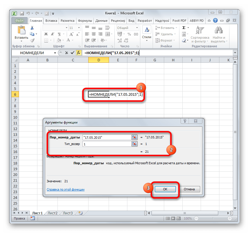
НОМНЕДЕЛИ

Предназначением оператора НОМНЕДЕЛИ является указание в заданной ячейке номера недели по вводной дате. Аргументами является собственно дата и тип возвращаемого значения. Если с первым аргументом все понятно, то второй требует дополнительного пояснения. Дело в том, что во многих странах Европы по стандартам ISO 8601 первой неделей года считается та неделя, на которую приходится первый четверг. Если вы хотите применить данную систему отсчета, то в поле типа нужно поставить цифру «2». Если же вам более по душе привычная система отсчета, где первой неделей года считается та, на которую приходится 1 января, то нужно поставить цифру «1» либо оставить поле незаполненным. Синтаксис у функции такой:

=НОМНЕДЕЛИ(дата;[тип])

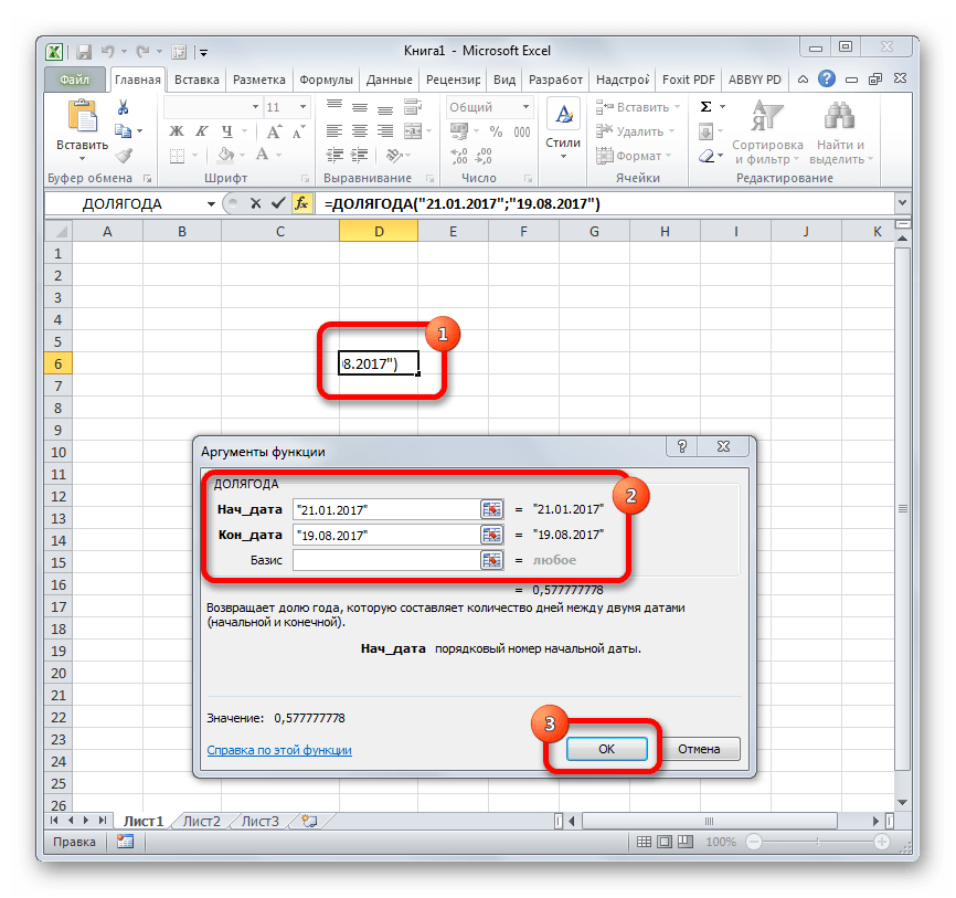
ДОЛЯГОДА

Оператор ДОЛЯГОДА производит долевой расчет отрезка года, заключенного между двумя датами ко всему году. Аргументами данной функции являются эти две даты, являющиеся границами периода. Кроме того, у данной функции имеется необязательный аргумент «Базис». В нем указывается способ вычисления дня. По умолчанию, если никакое значение не задано, берется американский способ расчета. В большинстве случаев он как раз и подходит, так что чаще всего этот аргумент заполнять вообще не нужно. Синтаксис принимает такой вид:

=ДОЛЯГОДА(нач_дата;кон_дата;[базис])

Мы прошлись только по основным операторам, составляющим группу функций «Дата и время» в Экселе. Кроме того, существует ещё более десятка других операторов этой же группы. Как видим, даже описанные нами функции способны в значительной мере облегчить пользователям работу со значениями таких форматов, как дата и время. Данные элементы позволяют автоматизировать некоторые расчеты. Например, по введению текущей даты или времени в указанную ячейку. Без овладения управлением данными функциями нельзя говорить о хорошем знании программы Excel.

Sometimes excel interprets date formats as a text string. Microsoft Excel has an inbuilt date formula that any frequent user of excel is aware of. It is the primary function used to calculate dates in Excel, and it can be used to extract a date from a text string. The date function in Excel is the Date and time function that returns a serial number in sequence format representing a valid date. This function’s beauty helps assemble dates that need to change dynamically based on other values in a data sheet. The formula is:

=DATE (year, month, day) where the arguments mean;

Year- It is a required argument of the function representing the number of the year of the Date. It is always expressed in four digits to avoid confusion.

Month- this is a required argument representing the number for the month of the year to use. It can be a + or – number which means the months from January (1) to December (12)

Day-it is also a required argument in Excel representing the number for the day or Date in a particular month.

It is a straightforward and more effortless function to use. Let’s get to know how to use an Excel date formula.

How to create and use date formula

1. Open your excel worksheet click where you need the Date created.

2. from the main menu ribbon, click on the Formulas tab.

3. Under the Function Library group, click on the drop-down arrow on the option Date& Time.

4. Select Date from the given options. Excel will display a dialog box.

5. Fill in the given fields representing the date formula.

6. Click OK. Your Date will be created and inserted into the selected cell.

Method 1: using the date formula to return a serial number for a date

For example, when you want to return a serial number that corresponds to March 14, 2021, you use the formula:

=DATE (2022, 2, 25)

But in cases where you do not want to specify the values that represent the year, month, and day directly in a formula, you can use all the arguments in other Excel date functions. You can decide to combine the YEAR and TODAY function as shown below to get a serial number:

=DATE (YEAR (TODAY ()), MONTH (TODAY ()), 14). The result will display a serial number for the fourteenth day of the current month and year.

 

Method 2: Using the date function to return Date based on values in other cells

When the values meant to create a date sequence are stored in different cells, all you have to do is use the date function. For example, when you have the year in cell A3, the month in cell B3, and the day in cell C3, you can use the function;

=DATE (A3, B3, C3)

Method 3: Using the date function to subtract or add dates in excel

To add or subtract some days from a given date, you first need to convert that Date into a serial number using the excel date function. For example, in the case of adding days to your date function, here is what you do;

=DATE (2022, 2, 25) + 10

When it comes to subtracting, replace the + sign with a minus sign.

Method 4: Using the date formula to convert a string of text or number to a date

The date function is beneficial when it comes to extracting Dates from a string of texts. Such scenarios occur when excel does not recognize the format used. The date function is used in liaison with other functions as stated below;

=DATE (RIGHT, MID, LEFT)

Using Date Formula to Insert Today’s Date

You can use the TODAY function to insert today’s date in any cell in Excel. The function takes no arguments but only returns today’s date. It is represented by the syntax below;

=TODAY()

The only downside is that the TODAY function is not updated automatically. Hence, if you want to update it, just press F9 or re-enter the formula. It also collects the present date from your computer; thus, it will also return a wrong date if the computer’s date is wrong.

Using Date Formula to Insert the First Day of Any Month

You can simply use 1 in place of any day argument to insert the first date of any month. It is represented by the syntax

=DATE(yy,mm,dd),  where;

dd is the first day of the month, usually represented by 1.

For example; to get the first day of June of 2022, the formula will be:

=DATE(2022,6,1)

However, it becomes a challenge to extract the first date of the month from any date. For instance, assuming you want to extract the first date of the month from 21-February-2020 in cell B4, you can use the formula below;

=B4-DAY(B4)+1

If you want to extract the first date of a month from another date, you can place the date inside the date function as shown below:

=DATE(2020,5,15)-DAY(DATE(2020,5,15))+1

In this case, the DAY function returns the day number of any date inserted into it. For example, DAY(DATE(2022,5,15))+1 will return 15. Since Excel accepts any date as a numerical value, you can add or subtract dates from Excel with any number. Therefore, the above formula subtracts 15 days from the date 1^st September 2022 and returns the last day of the previous month, 31-August-2022.

Using Date Formula to Insert the Last Day of Any Month

If you want to insert the last date of any month, enter the last day of that month in the day argument of the DATE function.

For example, to get the last date February 2022, the formula will be:

=DATE(2022,2,28)

However, to extract the last date of the month from any given date, you need to use the EOMONTH function, whose syntax is:

=EOMONTH(start_date,months), where;

Start_date is the last date of the month from which you want to extract the date.

Months denote the number of months you want to move forward. If you want to extract the last date of the present month, it will 0. For next month will be 1, and so on.

For example, if you want to get the last date of the month from 12-February-2022, you can use the formula below:

=EOMONTH(DATE(2022,2,12),0)

To get the last date of the month 3 months later, the formula will become:

=EOMONTH(DATE(2022,2,12),3)

Using Date Formula to Convert Date to Text

You can convert a date into text using the TEXT function of Excel with the following syntax:

=TEXT(value,format_text), where;

Value is the value you want to convert to text.

Format_text. Is the format in which you want the text to appear.

If you want to extract the names of the month of any date, you can use the formula below:

=TEXT(DATE(2022,3,20),»mmmm»)

where,

“mmmm” is the format for months.

Using Date Formula to Count Total Number of Workdays Between Two Dates

You can use the NETWORKDAYS function in excel to count the total number of work days between two days. The function is represented by the following generic formula:

=NETWORKDAYS(start_date,end_date,[holidays]), where;

Start_date is the first date.

 End_date is the ending date.

 [holidays] is a list of holidays.

For example; if you have a dataset with B4:B20 as a list of the holidays, you can get the total workdays between 1-January-2021 to 31-December-2022 using the following formula:

=NETWORKDAYS(DATE(2021,1,1),DATE(2022,12,31),B4:B20)

When you write the above formula in let’s say cell E4, you will get 510 as the total number of working days. However, to count the days without weekends, you use NETWORKDAYS.INTL function.

Using Date Formula to Determine the Workday After a Specific Number of Days

You can use the WORKDAY function in place of the NETWORKDAYS function to determine a specific date after a given number of workdays from a starting date. The function is represented by the syntax:

=WORKDAY(start_date,days,[holidays]), where;

Start_date is the starting date.

Days is the total number of workdays between the two dates.

 [holidays] is a list of holidays.

Using the above example where you have B4:B20 as a list of holidays. You can find out the workday after 1000 days starting from 1-January-2021 using the following formula:

=WORKDAY(DATE(2021,1,1),1000,B4:B20)

Using The Date Function to Create A Series Of Dates

You can also use the DATE function to create a series of dates with specific days’ intervals. For example, if you want to create interview dates with intervals of 7 days, with 20^th May 2021 as the first date, you can proceed with the following steps:

1. Enter the first date in the DATE formula. Assuming you want to use cell C4 as your first case, you can write this formula:

=DATE(2022,5,20)

2. Select all the cells in column C, go to the Home ribbon, and select Fill under the Editing list of options.

3. When you click on Fill, the drop-down menu will appear. Select Series.

4. A new Series dialogue will appear. Select Column from the Series selection, Date from the Type section, and Day from the Date Unit section.

5. Enter your interval between two dates in the Step Value. In this case, you have 7 days as your interval between two dates; hence, write 7.

6. Click OK and you see a series of interview dates displayed in the cells.

You can also use a formula to generate interview dates automatically, especially if you do not want to do it manually. In this case, the formula will be:

=DATE(2022,5,SEQUENCE(17,1,20,7))

where:

17 within the SEQUENCE function is the total number of days of the series (C4:C20).

20 is the starting date of May (20 May).

7 is the dates’ intervals.

Write the formula in cell C4 and click the Enter button. After that, you only use the Autofill Handle to drag the formula down the column to generate interview dates in the remaining cells. You can alter the formula based on your dataset. Also, remember that the SEQUENCE function is only available in Office 365.

Conclusion

From the article above, we get to know how to use Excel’s Date formula and how to create a date. The Date function has many more uses that are not mentioned above. I hope you find the information helpful.