
Excel for Microsoft 365 Excel 2021 Excel 2019 Excel 2016 Excel 2013 Excel 2010 Excel 2007 More…Less
Important: The calculated results of formulas and some Excel worksheet functions may differ slightly between a Windows PC using x86 or x86-64 architecture and a Windows RT PC using ARM architecture. Learn more about the differences.
Let’s say you want to find out how many inventory items are unprofitable (subtract profitable items from total inventory). Or, maybe you need to know how many employees are approaching retirement age (subtract the number of employees under 55 from total employees).
What do you want to do?
There are several ways to subtract numbers, including:
-
Subtract numbers in a cell
-
Subtract numbers in a range
Subtract numbers in a cell
To do simple subtraction, use the — (minus sign) arithmetic operator.
For example, if you enter the formula =10-5 into a cell, the cell will display 5 as the result.
Subtract numbers in a range
Adding a negative number is identical to subtracting one number from another. Use the SUM function to add negative numbers in a range.
Note: There is no SUBTRACT function in Excel. Use the SUM function and convert any numbers that you want to subtract to their negative values. For example, SUM(100,-32,15,-6) returns 77.
Example
Follow these steps to subtract numbers in different ways:
-
Select all of the rows in the table below, then press CTRL-C on your keyboard.
Data
15000
9000
-8000
Formula
=A2-A3
Subtracts 9000 from 15000 (which equals 6000)
-SUM(A2:A4)
Adds all number in the list, including negative numbers (net result is 16000)
-
In the worksheet, select cell A1, and then press CTRL+V.
-
To switch between viewing the results and viewing the formulas, press CTRL+` (grave accent) on your keyboard.Or, click the Show Formulas button (on the Formulas tab).
Using the SUM function
The SUM function adds all the numbers that you specify as arguments. Each argument can be a range, a cell reference, an array, a constant, a formula, or the result from another function. For example, SUM(A1:A5) adds all the numbers in the range of cells A1 through A5. Another example is SUM(A1, A3, A5) which adds the numbers that are contained in cells A1, A3, and A5 (A1, A3, and A5 are arguments).
Need more help?
The subtraction formula in excel facilitates the subtraction of numbers, cells, percentages, dates, matrices, times, and so on. It begins with the comparison operator “equal to” (=) followed by the first number, the minus sign, and the second number. For example, to subtract 2 and 5 from 15, apply the formula “=15-2-5.” It returns 8.
In subtraction, the first number is the minuend (from which a number has to be subtracted) and the second number is the subtrahend (the number to be subtracted). The resulting number is the difference.
The arithmetic operator “minus” (-) is placed between the minuend and the subtrahend.
Table of contents
- The Subtraction Formula of Excel
- How to Use the Subtraction Formula in Excel?
- Example #1
- Example #2
- The Rules Governing the Subtraction Excel Formula
- Frequently Asked Questions
- Recommended Articles
- How to Use the Subtraction Formula in Excel?
How to Use the Subtraction Formula in Excel?
The subtraction formula of Excel is easy to use. Let us go through the following examples to understand its working.
You can download this Subtraction Formula Excel Template here – Subtraction Formula Excel Template
Example #1
The following table shows some values in columns A and B. We want to subtract the values in column B from those of column A.
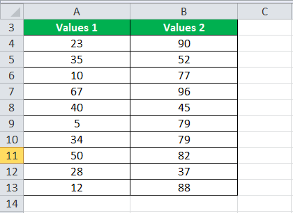
The steps to subtract the values of column B from those of column A are listed as follows:
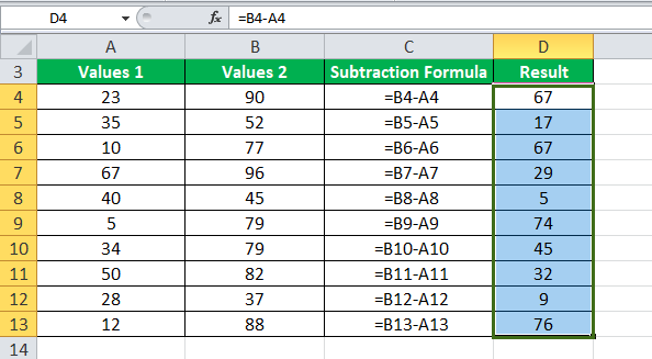
- Enter the comparison operator “equal to” (=), followed by the cell B4, the “minus” sign (-), and the cell A4. Press the “Enter” key. The output is 67.
Note: The references B4 and A4 can either be typed or selected by clicking on the respective cells.

- Apply the subtraction excel formula to the remaining values. Alternatively, drag the formula of C4 till C13, as shown in the following image.

- The final output appears, as shown in the following image. For simplicity, we have retained the formulas in column C and given the differences in column D.
Note: If the values in column A or column B change, the result is automatically updated in column D.


Example #2
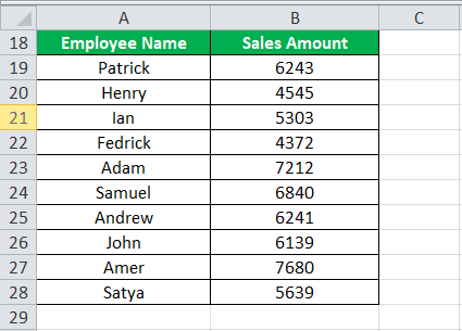
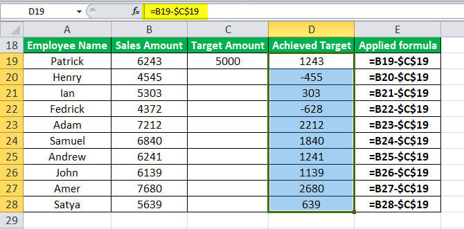
The following table shows the names and the revenuesRevenue is the amount of money that a business can earn in its normal course of business by selling its goods and services. In the case of the federal government, it refers to the total amount of income generated from taxes, which remains unfiltered from any deductions.read more generated (in Rs.) by ten employees of an organization. It has been decided to award Rs. 10,000 worth vouchers to those employees who have achieved the sales target of Rs. 5000.
Find the employees eligible for the reward.
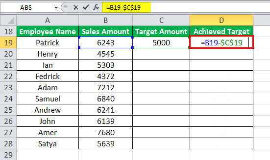
Step 1: Enter the following formula.
“=B19-$C$19”
To calculate the revenue generated over and above the target (Rs. 5000), we subtract the latter (column C) from the former (column B). Since the target amount is the same for all the employees, we use the absolute referenceAbsolute reference in excel is a type of cell reference in which the cells being referred to do not change, as they did in relative reference. By pressing f4, we can create a formula for absolute referencing.read more $C$19.
Note: In absolute cell reference, the dollar sign ($) is placed before the column letter and the row number like in $C$19. This keeps the column and the row constant.
Step 2: Press the “Enter” key. The final output appears in column D, as shown in the following image.
For simplicity, we have retained the formulas in column E and given the differences in column D. The employees who have negative difference values (column D) are not eligible for the reward.
Hence, Henry and Fedrick are not eligible while the rest of them receive the gift voucher.
The Rules Governing the Subtraction Excel Formula
- It always begins with the comparison operator “equal to” (=).
- It requires the insertion of the arithmetic operator “minus” (-) between two values.
- It is used in both, simple and advanced mathematical problems where a comparison between two values is required.
- It can be used in combination with other arithmetic operators like “plus” (+), “percent” (%), “forward slash” (/), “asterisk” (*), and so on.
Frequently Asked Questions
1. What is the subtraction formula of Excel and how to use it?
MS Excel does not have a SUBTRACT function. However, it facilitates subtraction by the insertion of the “minus” sign (-) between two values. The basic subtraction formula is stated as follows:
“=number 1-number 2”
The usage of the subtraction excel formula is listed in the following steps:
• Enter the comparison operator “equal to” (=).
• Enter the first number, followed by the “minus” sign (-), and the second number. Alternatively, select the cells containing values.
• Press the “Enter” key and the result appears in the cell where the formula was entered.
2. How to use the subtraction formula for multiple cells in Excel?
There are various ways of subtracting multiple cells from a single cell. For example, let us subtract the cells A12, A13, A14, and A15 from the cell A1.
Select any one of the following three methods:
• Apply the formula “=A1-A12-A13-A14-A15”.
• Apply the formula “=A1-SUM(A12:A15)”.
• Place the “minus” sign (-) before the numbers in cells A12, A13, A14, and A15. Apply the formula “=SUM(A1,A12:A15)”.
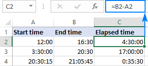
3. How to use the subtraction formula for calculating time in Excel?
To calculate time, apply the following formula:
“=End time-Start time”
For example, cells A6 and B6 contain 2:30:00 and 7:00:00 respectively. The number of hours in between the two times are calculated by the formula “=B6-A6”. The difference is 4:30:00.
Note: For correct results, apply the time format to the cell containing the formula.
Recommended Articles
This is a guide to the subtraction formula in Excel. Here we discuss how to subtract two numbers in excel with step by step examples. You can download the Excel templates from the website. For more on Excel, take a look at these functions –
- Excel NumberingNumbering in excel means providing a cell with numbers which are like serial numbers to some table, obviously it can also be done manually by filling first two cells with numbers and drag down to the end to table which excels will automatically fill the series.read more
- Equations in ExcelIn Excel, equations are the formulas we type into cells. We begin by writing an equation with an equals to symbol (=), which Excel knows as calculate.read more
- CAGR Formula in ExcelCAGR or compound annual growth rate calculates the growth rate of a particular amount annually. We make categories in tables and apply the formula to calculate CAGR. Formula = (Ending balance/Starting balance)˄(1/Number of years) – 1.read more
- Row Limit in ExcelLimit of rows in excel is a great tool to add more protection to the spreadsheet as this limits the other users to change or modify the spreadsheet to an extensive limit.read more
While Excel is an amazing tool for data analysis, many people use it for basic arithmetic calculations such as addition, subtraction, multiplication, and division.
If you’re new to Excel and wondering how to subtract in Excel, you’re at the right place.
In this tutorial, I will show you how to subtract in Excel (subtract cells, ranges, columns, and more).
I will start with the basics and then would cover some advanced subtraction techniques in Excel. I also cover how to subtract dates, times, and percentages in Excel.
So let’s get to it!
Subtracting Cells/Values in Excel
Let’s start with a really simple example, where I have two values (say 200 and 100) and I want to subtract these and get the result.
Here is how to do this:
- Select the cell where you want to subtract and enter an equal to sign (=)
- Enter the first value
- Enter the subtraction sign (minus sign -)
- Enter the second number
- Hit Enter

The above steps would perform the calculation in the cell and display the result.
Note that this is called a formula in Excel, where we start with an equal-to sign and then have the formula or the equation that we want to solve.
In the above example, we hard-coded the values in the cell. This means that we manually entered the values 200 and 100 in the cell.
You can also use a similar formula when you have these values in cells. In that case, instead of entering the values manually, you can use the reference of the cell.
Suppose you have two values in cell B1 and B2 (as shown below), and you want to subtract the value in cell B2 from the value in cell B1

Below is the formula that will do this:
=B1-B2

It’s the same construct, but instead of manually entering the values in the formula, we have used the cell reference which holds the value.
The benefit of doing this is that in case the values in the cells change, the formula would automatically update and show you the correct result.
Subtracting a Value from an Entire Column
Now let’s get to slightly more advanced subtraction calculations.
In the above example, we had two values that we wanted to subtract.
But what if you have a list of values in a column, and you want to subtract one specific value from that entire column.
Again, you can easily do that in Excel.
Suppose you have a data set as shown below and you want to subtract the value 10 from each cell in column A.

Below are the steps to do this:
- In cell B2, enter the formula: =A2-10

- Copy cell B2
- Select cell B3 to B12
- Paste the copied cell

When you do this, Excel will copy the formula in cell B2, and then apply that to all the cells where you pasted the copied cell.
And since we are using a cell reference in the formula (A2), Excel would automatically adjust the cell reference as it goes down.
For example, in cell B3, the formula would become =A3-10, and in cell B4, the formula would become A4-10.
If Using Microsoft 365
The method that I’ve covered above will work with all the versions of Excel, but if you using Microsoft 365, then you can use an even easier formula.
Suppose you have the same data (with data in column A) and you want to subtract 10 from each cell, you can use the below formula in cell B2:
=A2:A12-10

That’s it!
You don’t need to worry about copying and pasting the formula in other cells as Excel would take care of it.
This is called a dynamic array formula, where the result does not return one single value, but an array of values. And these are values are then spilled over to other cells in the column
Note: For these dynamic array formulas to work, you need to make sure the cells where the result would be populated are empty. In case there is already a number of text in these cells, you will see the #SPILL! error in the cell where you enter the formula.
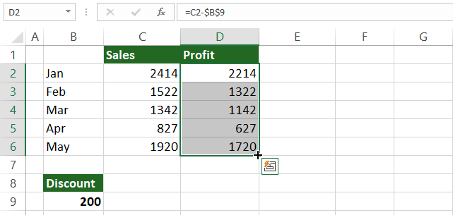
Subtracting a Cell Value from an Entire Column
In the above example, I subtracted 10 from multiple cells in a column.
We can use the same concept to subtract a value in a cell from an entire column.
Suppose you have a dataset as shown below where you want to subtract the value in cell D2 with all the cells in column A.

Below are the steps to do this:
- In cell C2, enter the formula: =A2-$D$2

- Copy cell C2
- Select cell C3 to C12
- Paste the copied cell

In this example, I have used the formula A2-$D$2, which makes sure that when I copy the formula for all the other cells in column C, the value that I am subtracting remains the same, which is cell B2.
When you add a dollar before the column alphabet and the row number, it makes sure that in case you copy the cell with this reference and paste it somewhere else, the reference would still remain $D$2. This is called absolute reference (as these don’t change).
When you copy this formula in cell C3, it would become A3-$D$2, and in cell C4, it would become A4-$D$2.
So while the first part of the reference keeps changing from A3 to A4 as we copy it down, the absolute reference doesn’t change,
This allows us to subtract the same value from all the cells in column A.
If Using Microsoft 365
If you’re using Microsoft 365 and have access to dynamic arrays, you can also use the below formula:
=A2:A12-D2

With dynamic arrays, you don’t have to worry about references changing. It will take care of it itself.
Subtract Multiple Cells From One Cell
Similar to the above example, you can also delete values in an entire column from a single value or the cell that holds the value.
Suppose you have a data set as shown below and you want to subtract all the values in column B from the value in cell A2.

Below are the steps to do this:
- In cell C2, enter the formula: =$A$2-B2
- Copy cell C2
- Select cell C3 to C12
- Paste the copied cell

The logic used here is exactly the same as above, where I’ve locked the reference $A$2 by adding a $ sign before the column alphabet and row number.
This way, the cell reference $A$2 doesn’t change when we copy it in column C, but the second reference of the formula (B2), keeps changing when we go down the cell.
If Using Microsoft 365
If you’re using Microsoft 365 and have access to dynamic arrays, you can also use the below formula:
=A2-B2:B12

Subtracting Cells in Two Columns
In most practical cases, you will have two columns where you want to subtract the cells in each column (in the same row) and get the result.
For example, suppose you have the Revenue and Expense values in two columns and you want to calculate the Net Income (which is the difference between revenue and expenses)

Here is how to do this:
- In cell C2, enter the formula: =B2-C2

- Copy cell C2
- Select cell C3 to C12
- Paste the copied cell

The above formula will automatically adjust the reference as it’s copied down and you will get the difference between Revenue and Expense in that row.
If Using Microsoft 365
The method that I’ve covered above will work with all the versions of Excel, but if you using Microsoft 365, then you can use an even easier formula.
Suppose you have the same data and you want to subtract the two columns, you can use the below formula:
=B2:B11-C2:C11
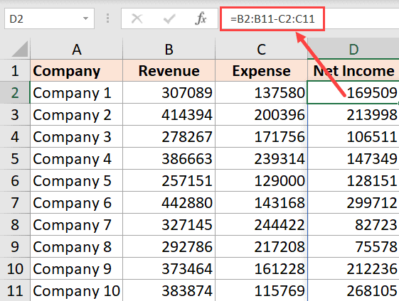
Note that this is made possible because Excel in Microsoft 365 has something called Dynamic Arrays. If you don’t have these, then it’s won’t be able to use this formula.
Subtract Dates in Excel
Dates and Time values are stores as numbers in the backend in Excel.
For example, 44197 represents the date 01 Jan 2021, and 44198 represents ṭhe date 2 Jan 2021.
This allows us to easily subtract dates in Excel and find the difference.
For example, if you have two dates, you can subtract these and find out how many days have elapsed between these two dates.
Suppose I have a dataset as shown below where I have the ‘Start Date’ and the ‘End Date’ and I want to find out the number of days between these two dates.

A simple subtraction formula would give me the result.
=B2-A2

There is a possibility that Excel will give you the result in the date format instead of a number as shown above.
This sometimes happens when Excel tries to be helpful and pick up the format from the adjacent column.
You can easily adjust this and get the values in numbers by going to the Home tab, and select General in the number format drop-down.
Note: This formula would only work when you using a date that Excel recognizes as a valid date format. For example, if you use 01.01.2020, Excel won’t recognize it as a date and consider it a text string. So you won’t be able to subtract dates with such a format
You can read more about subtracting dates in Excel here
Subtract Time in Excel
Just like dates, even time values are stored as numbers in Excel.
While the day part of the date would be represented by the whole number, the time part would be represented by the decimal.
For example, 44197.5 would represent 01 Jan 2021 12:00 PM and 44197.25 would represent 01 Jan 2021 09:00 AM
In case you have time values in Excel, what you really have in the back end in Excel are decimal numbers that represent that time value (which are formatted to be shown as time in the cells).
And since these are numbers, you can easily subtract these.
Below I have a data set where I have the start time and the end time, and I want to calculate the difference between these two times.

Here is the formula that will give us the difference between these time values:
=B2-A2

There is a high possibility that Excel will change the format of the result column to show the difference as a time value (for example, it may show you 9:00 AM instead of 0.375). You can easily change this by going to the Home tab and selecting General from the format dropdown.

Note that in case of times, you will get the value in decimals, but if you want it in hours, minutes, and seconds, you can do that by multiplying the decimal value with 24 (for getting hours), or 24*60 for getting minutes and 24*60*60 for getting seconds.
So if you want to know how many hours are there in the given time in our dataset, you can use the below formula:
=(B2-A2)*24

Subtract Percentages in Excel
Subtracting percentages from a number in Excel is a little different than subtracting two whole numbers or decimals.
Suppose you have two percentage values (as shown below) and you want to subtract one from another, you can use a simple subtraction formula

But if you want to subtract a percentage value from a non-percentage value, you need to do it differently.
Suppose you have 100 in cell B1 and you want to subtract 20% from this value (i.e., subtract 20% of 100 from 100).
You can use the below formal in this case:
=B1*(1-20%)

You can also use the below formula:
=B1-B1*20%
In case you have the percentage value in a cell, then you can use the cell reference as well. For example, if you have the dataset as shown below, and you want to subtract the percentage value in cell B2 from the number in B1.

Then you can use the below formula:
=B1-B1*B2

Subtract Using Paste Special
And finally, you can also use Paste Special trick to subtract in Excel.
This is useful when you want to quickly subtract a specific value from an entire column.
Suppose you have the dataset as shown below and you want to subtract 100 from each of these numbers.

Below are the steps to do this:
- In an empty cell, enter the value that you want to subtract from the entire column. In this example, I will enter this value in cell D1

- Copy cell D1 (which is the cell where you have entered this value you want to subtract)

- Select the entire column from which you want to subtract the copied value
- Right-click and then click on the Paste Special option

- In the special dialog box, select Values as the Paste option

- Under Operations, select Subtract

- Click OK
- Delete the value that you entered in the cell in Step 1
The above steps but simply subtract the value that you copied from the selected column. The result you get from this is a static value.

The benefit of this method is that you do not need an additional column where you need to apply a formula to subtract the values. In case you want to keep the original values as well, simply create a copy of the column and then use the above steps
So these are different ways that you can use Excel to subtract values/percentages, cells, and columns.
Understanding these basic concepts will help you use the Excel spreadsheet tool the most efficient way.
I hope you found this tutorial useful.
Other Excel tutorials you may also like:
- How to Add or Subtract Days to a Date in Excel (Shortcut + Formula)
- How to Multiply in Excel Using Paste Special
- How to Sum Only Positive or Negative Numbers in Excel
- Change Negative Number to Positive in Excel [Remove Negative Sign]
- How to Subtract Multiple Cells from One Cell in Excel
- Calculate Percentage Change in Excel (% Increase/Decrease Formula)
The tutorial shows how to use the subtraction formula in Excel. Learn how to subtract numbers, percentages, dates, and times easily.
This article is a part of our must-have guide on Excel Formulas.
Subtraction is a simple arithmetic operation. We all know that you will use the minus sign to subtract one number from another. Okay, how it works if you are using Microsoft Excel? What kind type of data can you subtract? Almost all: you can use numbers and percentages. Furthermore, subtraction is available for other data types like days, months, hours, minutes, and seconds. Believe it or not, you can use subtraction for texts too.
Let’s start and learn how to do it for almost all data types.
Table of contents:
- Excel Subtraction Formula
- How to Subtract cells in Excel
- Subtract multiple cells from one cell
- Subtraction formula for columns
- How to Subtract the same number from a column of numbers
- Subtraction formula for percentage
- How to subtract date and time in Excel
- Matrix subtraction formula (using arrays)
- How to subtract one text cell from another in Excel
Subtraction formula in Excel (apply minus sign)
In Excel, all formula starts with a ‘=’ (equal) sign. So, for example, to subtract two or more numbers, you need to apply the ‘-‘ sign (minus) operator between these values. That’s all, looks easy.
=number1 – number2
In the example, you want to subtract 33 from 50, use the simple formula and get 30 as the result of the equation:
=50 – 20
Steps to create the subtraction formula in Excel:
- Select the cell where you want to get the result and type an equal sign (=)
- Enter the first number
- Type the minus sign
- Add the second number
- Press Enter to evaluate the formula
Tip: you can do multiple subtractions within one basic formula.
In the example, you want to subtract more than one number from 50. To do that, separate the numbers using a minus sign.
=50 – 20 – 10 – 5
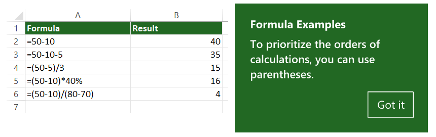
To prioritize the orders of calculations, you can use parentheses, like the example below:
=(50 – 10) / (10 – 5)
Let’s see a few formula examples:
How to Subtract cells in Excel
To execute a formula that subtracts one cell from another, use cell references:
=cell1 – cell2
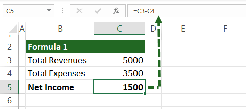
The following example shows how to subtract the number in cell C4 from the number in C3.
=C3 – C4
Forget to enter the cell references manually!
Instead, here are the steps to use subtraction between cells:
- Select the output cell
- Type an equals sign (=)
- Click on the cell that contains the minuend (C3)
- Type a minus sign (-)
- Click on the cell that contains the subtractor (C4)
- Press Enter to calculate the difference
Subtract multiple cells from one cell
There are three methods:
- use the SUM function
- apply the minus sign
- sum negative numbers.
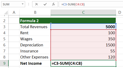
Example 1: Using the SUM function
The easiest way to subtract multiple cells from one is using the SUM function. First, add the subtrahends (C4:C8), then subtract from the minuend, in the example, cell C3.
=C3 – SUM(C4:C8)
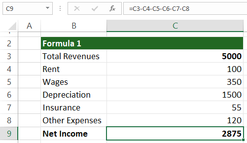
Example 2: Using the Minus sign
If you don’t want to use formulas, use the minus sign to subtract multiple numbers. In the example, you subtract cells C4:C8 from C3:
=C3 – C4 – C5 – C6 – C7 – C8
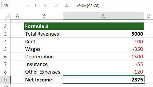
Example 3. The subtraction formula summarizes negative numbers
If you subtract a negative number from a positive number, the result will be the same as adding it. Use the SUM function to sum the positive and negative numbers.
=SUM(C3:C8)
Subtraction Formula for columns
The following example will show how to write a formula to subtract columns.
To subtract numbers from column D from the numbers in column C, enter the formula. But first, create a new column for the result in cell E2.
Type the formula for cell E2.
=C2-D2
After that, select cell E2 and copy the formula down using the cross sign.
In this case, we are talking about relative references.
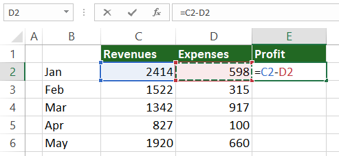
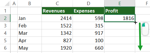
How to Subtract the same number from a column of numbers
In this example, you will use a fixed cell value, B9, as a subtrahend.
Steps to create a subtraction formula for cell D2:
- Select cell D2
- Type an equal sign
- Select cell C2
- Add a minus (-) sign
- Select cell B9
- Press F4
=C2 – $B$9
What’s the point? If you lock the cell using the dollar sign ($), you can create an absolute cell reference in Excel. From now on, the second part of the subtraction formula will fix.
Copy the formula down, and the result is correct in each row.
As a result of using absolute reference, the formula in cell D3 will change to =C3-$B$9, and so on.
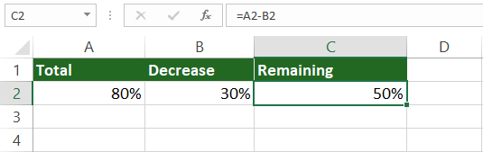
Subtraction formula for percentages
The subtraction between percentages is not rocket science, and the above-mentioned subtraction formula works fine. In the case of fixed values, use the classic method:
= 80% – 30%
You can use cell references, too by using the following formula:
= A2 – B2
How to decrease a number by a percentage
In the example, you want to subtract a percentage from a number.
The formula looks like this:
=Number * (1- %)
For example, let us see how you can reduce the number in B3 by 25%.
Use the formula:
= B3 * (1-$C$3)
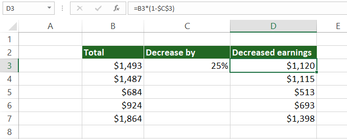
Because we are using absolute reference, it’s easy to copy the subtraction formula down.
How to subtract date and time in Excel
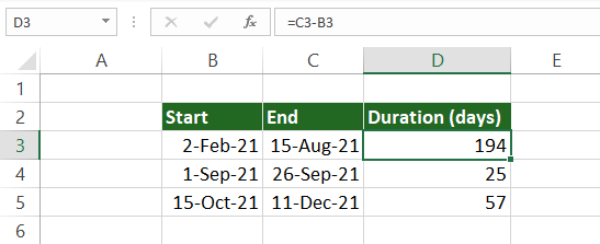
Subtraction formula for dates
Working with dates, it’s easy if you want to subtract one cell from the other. In the example, we would like to get dates in column D. The start and end dates are in cells B3 and C3.
To get the differences between two cells that contain date formats, use the minus sign in the subtraction formula:
= end_date – start_date
= C3 – B3
You’ll get the result in days.
Tip: It’s possible to subtract dates using built-in Excel functions. Use the DATE function to calculate the differences between dates!
The subtraction formula:
=DATE(2021,9,15) – DATE(2021,9,11) = 4
How to subtract time in Excel
You can create a time subtraction formula in Excel based on the date formula:
The syntax:
= end_time – start_time
= C3 – B3
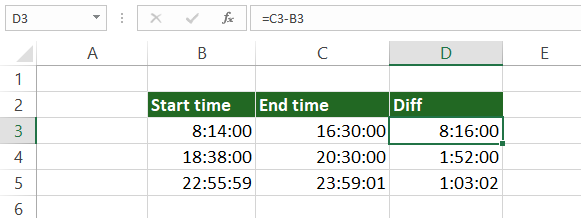
Now you have the result in D3. Copy the formula down to fill the column.
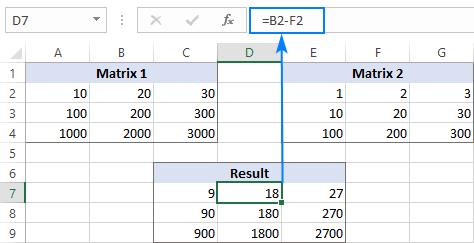
Matrix subtraction formula in Excel (using arrays)
Suppose that you have two matrices (with equal size), and you want to subtract the corresponding elements of the range.
For the sake of simplicity, here is an example:
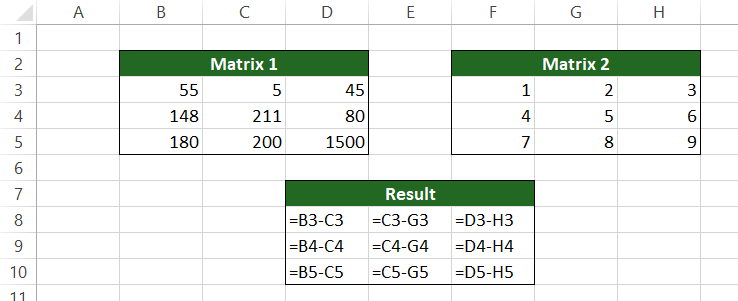
This method is a bit slow, so we are looking for a faster and better solution.
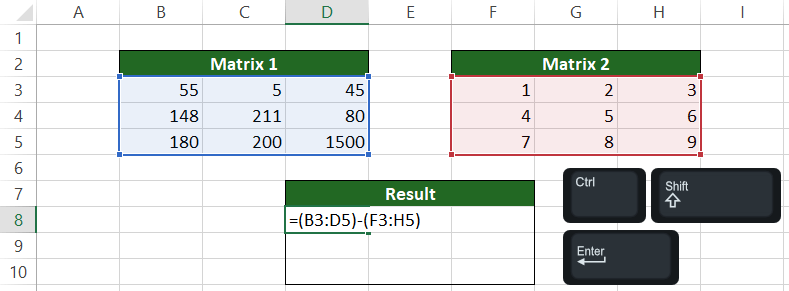
Steps to subtract matrix2 from matrix1 using an array formula!
- Select cell D8
- Enter the formula = (B3-D5) – (F3:H5)
- Use the Ctrl + Shift + Enter to create an array formula
Let us see the results of the subtraction In cell D8! Check the formula bar! The subtraction formula is surrounded by {curly brackets}.
Copy the formula to fill the remaining cells.
How to subtract one text cell from another in Excel?
If you are familiar with VBA, we have some good news. Use the TEXTSUBTRACT function to subtract characters in one string from another string:
Function textSubtract(startString As String, subtractString As String) As String


Dim charCounter As Integer
For charCounter = 1 To Len(subtractString)

  startString = Replace(startString, Mid(subtractString, charCounter, 1), "")

      Next charCounter

  textSubtract = startString

End Function
How to add a new code? First, open a new Workbook, and press Alt + F11 to open the VBE window. Then, insert a new module and add the code as mentioned above. Finally, save the Workbook in .xlsm format.
Tip: if you have found the ‘Excel found a problem with formula references in this Worksheet,’ try to fix it using absolute references.
In this article, we will learn how to apply Subtraction in Excel.
Scenario:
Subtraction is one of the four basic arithmetic operations, and every primary school pupil knows that to subtract one number from another you use the minus sign. This good old method works in Excel too. What kind of things can you subtract in your worksheets? Just any things which excel understands as numbers: such as numbers, percentages, days, months, hours, minutes and seconds.
Subtraction formula in Excel (minus formula)
You can even subtract matrices, text strings and lists. Now, let’s take a look at how you can do all this.
Manual Subtract in Excel
Subtract cells in Excel
Subtract columns
Subtract percentage
Subtracting dates
Subtracting times
Matrix subtraction
Let’s learn each of the above mentioned methods taking one by one to understand how subtraction works in excel.
Example :
All of these might be confusing to understand. Let’s understand how to use the function using an example. Here To perform a simple subtraction operation, you use the minus sign (-).
The basic Excel subtraction formula is as simple as this:
=number1-number2
For example, to subtract 10 from 100, write the below equation and get 90 as the result:
=100-10
To enter the formula in your worksheet, do the following steps:
In a cell where you want the result to appear, type the equality sign (=).
Type the first number followed by the minus sign followed by the second number.
Complete the formula by pressing the Enter key.
Like in math, you can perform more than one arithmetic operation within a single formula.
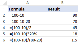
For example, to subtract a few numbers from 100, type all those numbers separated by a minus sign:
=100-10-20-30
To indicate which part of the formula should be calculated first, use parentheses. For example:
=(100-10)/(80-20)
The screenshot below shows a few more formulas to subtract numbers in Excel:
How to subtract cells in Excel
To subtract one cell from another, you also use the minus formula but supply cell references instead of actual numbers:
=cell_1 — cell_2
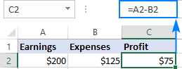
For example, to subtract the number in B2 from the number in A2, use this formula:
=A2-B2
You do not necessarily have to type cell references manually, you can quickly add them to the formula by selecting the corresponding cells. Here’s how:
In the cell where you want to output the difference, type the equals sign (=) to begin your formula.
Click on the cell containing a minuend (a number from which another number is to be subtracted). Its reference will be added to the formula automatically (A2).
Type a minus sign (-).
Click on the cell containing a subtrahend (a number to be subtracted) to add its reference to the formula (B2).
Press the Enter key to complete your formula.
And you will have a result similar to this:
How to subtract multiple cells from one cell in Excel
To subtract multiple cells from the same cell, you can use any of the following methods.
Method 1. Minus sign
Simply type several cell references separated by a minus sign like we did when subtracting multiple numbers.
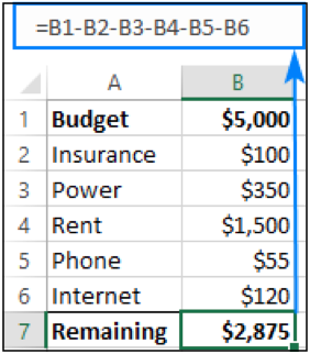
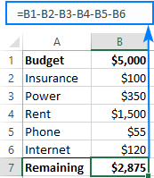
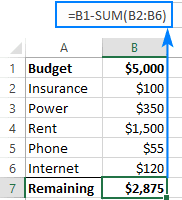
For example, to subtract cells B2:B6 from B1, construct a formula in this way:
=B1-B2-B3-B4-B5-B6
Method 2. SUM function
To make your formula more compact, add up the subtrahends (B2:B6) using the SUM function, and then subtract the sum from the minuend (B1):
=B1-SUM(B2:B6)
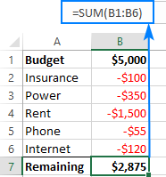
Method 3. Sum negative numbers
As you may remember from a math course, subtracting a negative number is the same as adding it. So, make all the numbers you want to subtract negative (for this, simply type a minus sign before a number), and then use the SUM function to add up the negative numbers:
=SUM(B1:B6)
How to subtract columns in Excel
To subtract 2 columns row-by-row, write a minus formula for the topmost cell, and then drag the fill handle or double-click the plus sign to copy the formula to the entire column.
As an example, let’s subtract numbers in column C from the numbers in column B, beginning with row 2:
=B2-C2
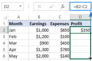
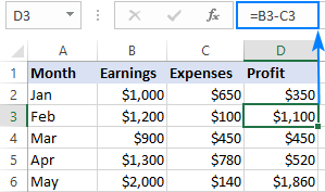
Due to the use of relative cell references, the formula will adjust properly for each row:
Subtract the same number from a column of numbers
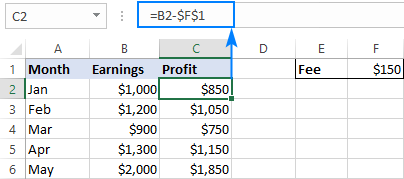
To subtract one number from a range of cells, enter that number in some cell (F1 in this example), and subtract cell F1 from the first cell in the range:
=B2-$F$1
The key point is to lock the reference for the cell to be subtracted with the $ sign. This creates an absolute cell reference that does not change no matter where the formula is copied. The first reference (B2) is not locked, so it changes for each row.
As the result, in cell C3 you will have the formula =B3-$F$1; in cell C4 the formula will change to =B4-$F$1, and so on:
If the design of your worksheet does not allow for an extra cell to accommodate the number to be subtracted, nothing prevents you from hardcoding it directly in the formula:
=B2-150
How to subtract percentage in Excel
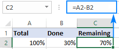
If you want to simply subtract one percentage from another, the already familiar minus formula will work a treat. For example:
=100%-30%
Or, you can enter the percentages in individual cells and subtract those cells:
=A2-B2
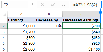
If you wish to subtract percentage from a number, i.e. decrease number by percentage, then use this formula:
=Number * (1 — %)
For example, here’s how you can reduce the number in A2 by 30%:
=A2*(1-30%)
Or you can enter the percentage in an individual cell (say, B2) and refer to that cell by using an absolute reference:
=A2*(1-$B$2)
For more information, please see How to calculate percentage in Excel.
How to subtract dates in Excel
The easiest way to subtract dates in Excel is to enter them in individual cells, and subtract one cell from the other:
=End_date — Start_date
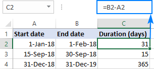
You can also supply dates directly in your formula with the help of the DATE or DATEVALUE function. For example:
=DATE(2018,2,1)-DATE(2018,1,1)
=DATEVALUE(«2/1/2018»)-DATEVALUE(«1/1/2018»)
More information about subtracting dates can be found here:
How to add and subtract dates in Excel
How to calculate days between dates in Excel
How to subtract time in Excel
The formula for subtracting time in Excel is built in a similar way:
=End_time-Start_time
For example, to get the difference between the times in A2 and B2, use this formula:
=A2-B2
For the result to display correctly, be sure to apply the Time format to the formula cell:
You can achieve the same result by supplying the time values directly in the formula. For Excel to understand the times correctly, use the TIMEVALUE function:
=TIMEVALUE(«4:30 PM»)-TIMEVALUE(«12:00 PM»)
For more information about subtracting times, please see:
How to calculate time in Excel
How to add & subtract time to show over 24 hours, 60 minutes, 60 seconds
How to do matrix subtraction in Excel
Suppose you have two sets of values (matrices) and you want to subtract the corresponding elements of the sets like shown in the screenshot below:
Here’s how you can do this with a single formula:
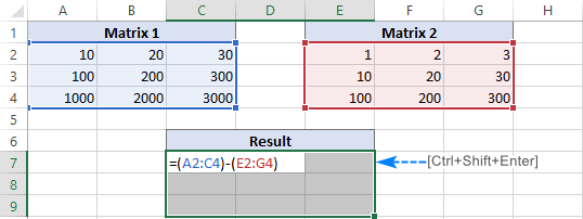
Select a range of empty cells that has the same number of rows and columns as your matrices.
In the selected range or in the formula bar, type the matrix subtraction formula:
=(A2:C4)-(E2:G4) , Now press Ctrl + Shift + Enter to make it an array formula.
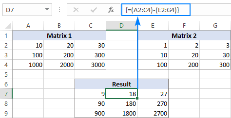
The results of the subtraction will appear in the selected range. If you click on any cell in the resulting array and look at the formula bar, you will see that the formula is surrounded by {curly braces}, which is a visual indication of array formulas in Excel:
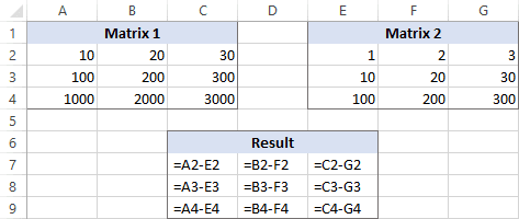
If you do not like using array formulas in your worksheets, then you can insert a normal subtraction formula in the top leftmost cell and copy in rightwards and downwards to as many cells as your matrices have rows and columns.
In this example, we could put the below formula in C7 and drag it to the next 2 columns and 2 rows:
=A2-C4
Due to the use of relative cell references (without the $ sign), the formula will adjust based on a relative position of the column and row where it is copied:
Subtract text of one cell from another cell
Here are all the observational notes using the formula in Excel
Notes :
- The subtract methods only apply to numbers not text.
- Now you can subtract any value in excel using the explained procedure.
Hope this article about How to use Subtraction in Excel is explanatory. Find more articles on calculating values and related Excel formulas here. If you liked our blogs, share it with your friends on Facebook. And also you can follow us on Twitter and Facebook. We would love to hear from you, do let us know how we can improve, complement or innovate our work and make it better for you. Write to us at info@exceltip.com.
Related Articles :
How to get Addition in Excel : Perform addition in Excel using SUM function or + (plus sign) in Excel.
How to get Multiplication in Excel : Perform addition in Excel using PRODUCT function or * (asterisk sign) in Excel
How to get Dividation in Excel : Perform addition in Excel using DIVIDE function in Excel.
How to get Quotient in Excel : Perform addition in Excel using divide option or / in Excel.
How to get Remainder in Excel : Perform addition in Excel using MOD function in Excel.
Popular Articles :
50 Excel Shortcuts to Increase Your Productivity : Get faster at your tasks in Excel. These shortcuts will help you increase your work efficiency in Excel.
How to use the VLOOKUP Function in Excel : This is one of the most used and popular functions of excel that is used to lookup value from different ranges and sheets.
How to use the IF Function in Excel : The IF statement in Excel checks the condition and returns a specific value if the condition is TRUE or returns another specific value if FALSE.
How to use the SUMIF Function in Excel : This is another dashboard essential function. This helps you sum up values on specific conditions.
How to use the COUNTIF Function in Excel : Count values with conditions using this amazing function. You don’t need to filter your data to count specific values. Countif function is essential to prepare your dashboard.