
Excel for Microsoft 365 Excel for Microsoft 365 for Mac Excel for the web Excel 2021 Excel 2021 for Mac Excel 2019 Excel 2019 for Mac Excel 2016 Excel 2016 for Mac Excel 2013 Excel 2010 Excel 2007 Excel for Mac 2011 More…Less
Multiplying and dividing in Excel is easy, but you need to create a simple formula to do it. Just remember that all formulas in Excel begin with an equal sign (=), and you can use the formula bar to create them.
Multiply numbers
Let’s say you want to figure out how much bottled water that you need for a customer conference (total attendees × 4 days × 3 bottles per day) or the reimbursement travel cost for a business trip (total miles × 0.46). There are several ways to multiply numbers.
Multiply numbers in a cell
To do this task, use the * (asterisk) arithmetic operator.
For example, if you type =5*10 in a cell, the cell displays the result, 50.
Multiply a column of numbers by a constant number
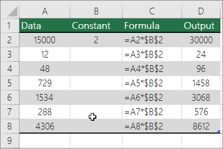
Suppose you want to multiply each cell in a column of seven numbers by a number that is contained in another cell. In this example, the number you want to multiply by is 3, contained in cell C2.
-
Type =A2*$B$2 in a new column in your spreadsheet (the above example uses column D). Be sure to include a $ symbol before B and before 2 in the formula, and press ENTER.
Note: Using $ symbols tells Excel that the reference to B2 is «absolute,» which means that when you copy the formula to another cell, the reference will always be to cell B2. If you didn’t use $ symbols in the formula and you dragged the formula down to cell B3, Excel would change the formula to =A3*C3, which wouldn’t work, because there is no value in B3.
-
Drag the formula down to the other cells in the column.
Note: In Excel 2016 for Windows, the cells are populated automatically.
Multiply numbers in different cells by using a formula
You can use the PRODUCT function to multiply numbers, cells, and ranges.
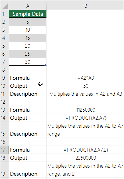
You can use any combination of up to 255 numbers or cell references in the PRODUCT function. For example, the formula =PRODUCT(A2,A4:A15,12,E3:E5,150,G4,H4:J6) multiplies two single cells (A2 and G4), two numbers (12 and 150), and three ranges (A4:A15, E3:E5, and H4:J6).
Divide numbers
Let’s say you want to find out how many person hours it took to finish a project (total project hours ÷ total people on project) or the actual miles per gallon rate for your recent cross-country trip (total miles ÷ total gallons). There are several ways to divide numbers.
Divide numbers in a cell
To do this task, use the / (forward slash) arithmetic operator.
For example, if you type =10/5 in a cell, the cell displays 2.
Important: Be sure to type an equal sign (=) in the cell before you type the numbers and the / operator; otherwise, Excel will interpret what you type as a date. For example, if you type 7/30, Excel may display 30-Jul in the cell. Or, if you type 12/36, Excel will first convert that value to 12/1/1936 and display 1-Dec in the cell.
Note: There is no DIVIDE function in Excel.
Divide numbers by using cell references
Instead of typing numbers directly in a formula, you can use cell references, such as A2 and A3, to refer to the numbers that you want to divide and divide by.
Example:
The example may be easier to understand if you copy it to a blank worksheet.
How to copy an example
-
Create a blank workbook or worksheet.
-
Select the example in the Help topic.
Note: Do not select the row or column headers.

Selecting an example from Help
-
Press CTRL+C.
-
In the worksheet, select cell A1, and press CTRL+V.
-
To switch between viewing the results and viewing the formulas that return the results, press CTRL+` (grave accent), or on the Formulas tab, click the Show Formulas button.

|
A |
B |
C |
|
|
1 |
Data |
Formula |
Description (Result) |
|
2 |
15000 |
=A2/A3 |
Divides 15000 by 12 (1250) |
|
3 |
12 |
Divide a column of numbers by a constant number
Suppose you want to divide each cell in a column of seven numbers by a number that is contained in another cell. In this example, the number you want to divide by is 3, contained in cell C2.
|
A |
B |
C |
|
|
1 |
Data |
Formula |
Constant |
|
2 |
15000 |
=A2/$C$2 |
3 |
|
3 |
12 |
=A3/$C$2 |
|
|
4 |
48 |
=A4/$C$2 |
|
|
5 |
729 |
=A5/$C$2 |
|
|
6 |
1534 |
=A6/$C$2 |
|
|
7 |
288 |
=A7/$C$2 |
|
|
8 |
4306 |
=A8/$C$2 |
-
Type =A2/$C$2 in cell B2. Be sure to include a $ symbol before C and before 2 in the formula.
-
Drag the formula in B2 down to the other cells in column B.
Note: Using $ symbols tells Excel that the reference to C2 is «absolute,» which means that when you copy the formula to another cell, the reference will always be to cell C2. If you didn’t use $ symbols in the formula and you dragged the formula down to cell B3, Excel would change the formula to =A3/C3, which wouldn’t work, because there is no value in C3.
Need more help?
You can always ask an expert in the Excel Tech Community or get support in the Answers community.
See Also
Multiply a column of numbers by the same number
Multiply by a percentage
Create a multiplication table
Calculation operators and order of operations
Need more help?
Want more options?
Explore subscription benefits, browse training courses, learn how to secure your device, and more.
Communities help you ask and answer questions, give feedback, and hear from experts with rich knowledge.
There is no in-built multiplication formula in Excel. Multiplication in excel is performed by entering the comparison operator “equal to” (=), followed by the first number, the “asterisk” (*), and the second number. In this way, it is possible to carry out the multiplication operation for a cell, row or column. For example, the formula “=16*3*2” multiplies the numbers 16, 3, and 2. It returns 96.
The arithmetic operator “asterisk” (*) is known as the multiplication symbol. It is placed between the numbers to be multiplied.
In multiplication, the number to be multiplied is known as the multiplicand. The number by which the multiplicand is multiplied is known as the multiplier. The multiplier and the multiplicand are also called factors. Their output of multiplication is known as the product.
In Excel, multiplication can be performed in the following ways:
- With the “asterisk” symbol (*)
- With the PRODUCT functionProduct excel function is an inbuilt mathematical function which is used to calculate the product or multiplication of the given numbers. If you provide this formula arguments as 2 and 3 as =PRODUCT(2,3) then the result displayed is 6.read more
- With the SUMPRODUCT functionThe SUMPRODUCT excel function multiplies the numbers of two or more arrays and sums up the resulting products.read more
Note: The SUMPRODUCT function multiplies and then sums the resulting products.
Table of contents
- How to Use Multiply Formula in Excel?
- Example #1 – Multiply Excel Columns With the “Asterisk”
- Example #2 – Multiply Excel Rows With the “Asterisk”
- Example #3 – Multiply With the PRODUCT Function
- Example #4 – Multiply and Sum With the SUMPRODUCT Function
- Example #5 – Multiply With Percentages
- Frequently Asked Questions
- Recommended Articles
How to Use Multiply Formula in Excel?
You can download this Multiply Function Excel Template here – Multiply Function Excel Template
Example #1 – Multiply Excel Columns With the “Asterisk”
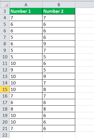
The following table shows two columns titled “number 1” and “number 2.” We want to multiply the numerical values of the first column by the second one.
Step 1: Enter the multiplication formula in excel “=A4*B4” in cell C4.
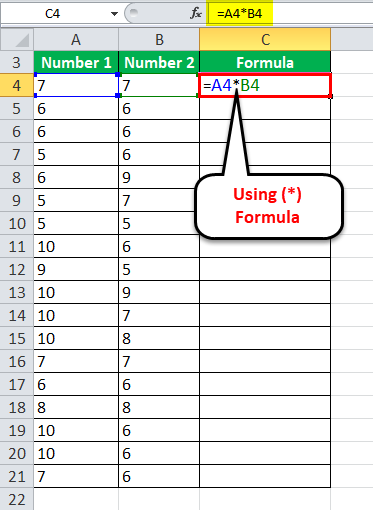
Step 2: Press the “Enter” key. The output is 49, as shown in the succeeding image. Drag or copy-paste the formula to the remaining cells.
For simplicity, we have retained the formulas in column C and given the products in column D.

Example #2 – Multiply Excel Rows With the “Asterisk”
The following table shows two rows titled “number 1” and “number 2.” We want to multiply the numerical values of the first row by the second one.
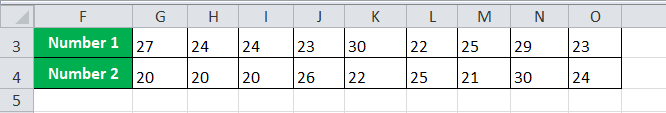
Step 1: Enter the multiplication formula “=G3*G4” in cell G5.
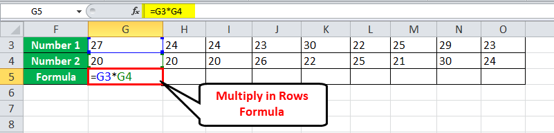
Step 2: Press the “Enter” key. The output is 540, as shown in the succeeding image. Drag or copy-paste the formula to the remaining cells.
For simplicity, we have retained the formulas in row 5 and given the products in row 6.

Example #3 – Multiply With the PRODUCT Function
The PRODUCT function can be given a list of numbers as arguments to be multiplied.
Working on the data of example #1, we want to multiply the numerical values of the two columns with the help of the PRODUCT function.
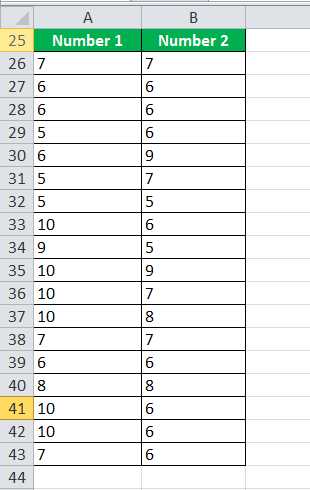
Step 1: Enter the formula “=PRODUCT (A26,B26)” in cell C26.

Step 2: Press the “Enter” key. The output is 49, as shown in the succeeding image. Drag or copy-paste the formula to the remaining cells.
For simplicity, we have retained the formulas in column C and given the products in column D.

Example #4 – Multiply and Sum With the SUMPRODUCT Function
With the SUMPRODUCT function, the numbers of two columns or rows are multiplied and the resulting products are summed up.
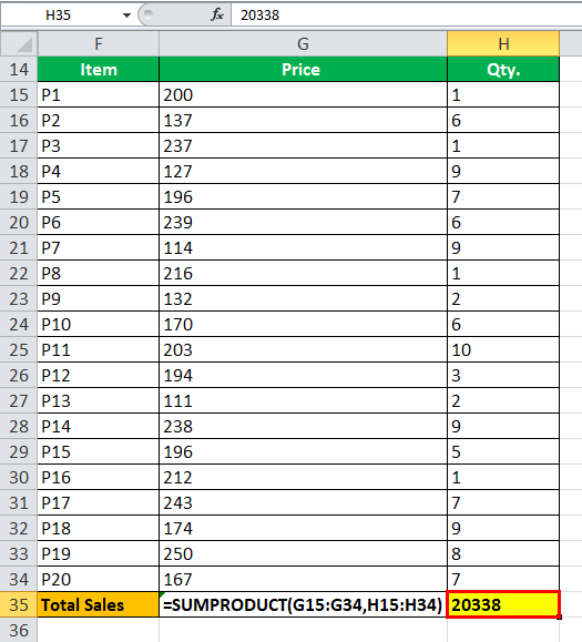
The following table shows the prices (in $ per unit) and quantities sold of 20 items. We want to calculate the total sales revenue generated by the organization.

Step 1: Enter the formula “=SUMPRODUCT (G15:G34,H15:H34).”
To calculate the sales revenue, the prices are multiplied by the quantity sold. Thereafter, the resulting products are added by the given formula.
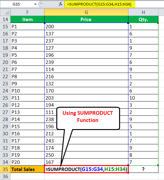
Step 2: Press the “Enter” key. The output is $20,338.
For simplicity, we have retained the formula in cell G35 and given the result in cell H35.
Example #5 – Multiply With Percentages
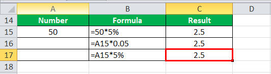
The following table shows a number in column A. We want to multiply this by 5%.
Step 1: Enter any of the following three formulas:
- “=50*5%”
- “=A15*0.05”
- “=A15*5%”

Step 2: Press the “Enter” key. The output is 2.5 with all the three formulas. It is shown in the following image.
For simplicity, we have retained the formulas in column B and given the results in column C.
Frequently Asked Questions
1. What is the multiplication formula and how to multiply in Excel?
There is no universal formula for multiplication in Excel. However, Excel facilitates multiplication with the use of the “asterisk” (*) and the PRODUCT function.
The formula using the “asterisk” is stated as follows:
“=number 1*number 2”
This is the simplest approach to multiplication that helps multiply numbers, cell references, rows, and columns.
The syntax using the PRODUCT function is stated as follows:
“=PRODUCT(number1,[number2], …)”
The “number1” and “number2” arguments can be in the form of numbers, cell references or ranges. Only the “number1” argument is required.
The steps to multiply in Excel are listed as follows:
• Enter the comparison operator “equal to” (=).
• Enter the multiplication formula.
• Press the “Enter” key to obtain the output.
Note: A maximum of 255 arguments can be provided to the PRODUCT function.
2. How to multiply in Excel without using the formula?
Let us multiply the numbers 4, 15, 23, and 54 (in the range A2:A5) by the constant 2 (in cell B2) without using the formula.
The steps to multiply in excel with “paste special” are listed as follows:
• Select cell B2 and press the keys “Ctrl+C” to copy it.
• Select the range A2:A5, which is to be multiplied.
• Right-click the selected range and choose “paste special.”
• In the “paste special” window, select “multiply” under “operation.”
• Click “Ok.”
The outputs 8, 30, 46, and 108 are obtained in the range A2:A5.
Note: If you do not want the range A2:A5 to be overridden with new values, copy-paste the numbers of this range to a separate column. This is to be done at the beginning of the mentioned procedure.
3. How to multiply two columns in Excel?
Let us multiply column A consisting of 5, 18, 26, and 44 (in the range A2:A5) by column B consisting of 6, 4, 9, and 2 (in the range B2:B5).
The steps to multiply two columns in excel using the multiplication symbol or the PRODUCT formula are listed as follows:
• Enter the formula “=A2*B2” or “=PRODUCT(A2,B2)” in cell C2.
• Press the “Enter” key. The output 30 appears in cell C2.
• Drag or copy-paste the formula to the remaining cells.
The outputs 30, 72, 234, and 88 are obtained in the range C2:C5.
Note: Since relative references are being used, the cell reference changes as the formula is copied.
The steps to multiply two excel columns using the array formula are listed as follows:
• Select the entire range C2:C5 where you want the output.
• Enter the formula “=A2:A5*B2:B5” in the selected range.
• Press the keys “Ctrl+Shift+Enter” together. The curly braces {} appear in the formula bar.
The outputs 30, 72, 234, and 88 are obtained in the range C2:C5.
Recommended Articles
This has been a guide to the multiply formula of Excel. Here we discuss how to multiply numbers, rows, columns, and percentages in Excel. We also discussed the usage of the PRODUCT and the SUMPRODUCT function of Excel. You may learn more about Excel from the following articles-
- SUMIFS With Multiple Criteria
- Formula Grade in ExcelThe Grade system formula is actually a nested IF formula in excel that checks certain conditions and returns the particular Grade if the condition is met. It is developed to check all conditions we have for the grade slab, and the grade that belongs to the condition is returned. read more
- SUMPRODUCT with Multiple CriteriaIn Excel, using SUMPRODUCT with several Criteria allows you to compare different arrays using multiple criteria.read more
- Excel Percentage Change FormulaA percentage change formula in excel evaluates the rate of change from one value to another. It is computed as the percentage value of dividing the difference between current and previous values by the previous value.read more
- Compare Two Lists in ExcelThe five different methods used to compare two lists of a column in excel are — Compare Two Lists Using Equal Sign Operator, Match Data by Using Row Difference Technique, Match Row Difference by Using IF Condition, Match Data Even If There is a Row Difference, Partial Matching Technique.read more
To multiply numbers in Excel, use the asterisk symbol (*) or the PRODUCT function. Learn how to multiply columns and how to multiply a column by a constant.
1. The formula below multiplies numbers in a cell. Simply use the asterisk symbol (*) as the multiplication operator. Don’t forget, always start a formula with an equal sign (=).

2. The formula below multiplies the values in cells A1, A2 and A3.

3. As you can imagine, this formula can get quite long. Use the PRODUCT function to shorten your formula. For example, the PRODUCT function below multiplies the values in the range A1:A7.

4. Here’s another example.

Explanation: =A1*A2*A3*A4*A5*A6*A7*B1*B2*B3*B4*C1*8 produces the exact same result.
Take a look at the screenshot below. To multiply two columns together, execute the following steps.
5a. First, multiply the value in cell A1 by the value in cell B1.

5b. Next, select cell C1, click on the lower right corner of cell C1 and drag it down to cell C6.

Take a look at the screenshot below. To multiply a column of numbers by a constant number, execute the following steps.
6a. First, multiply the value in cell A1 by the value in cell A8. Fix the reference to cell A8 by placing a $ symbol in front of the column letter and row number ($A$8).

6b. Next, select cell B1, click on the lower right corner of cell B1 and drag it down to cell B6.

Explanation: when we drag the formula down, the absolute reference ($A$8) stays the same, while the relative reference (A1) changes to A2, A3, A4, etc.
If you’re not a formula hero, use Paste Special to multiply in Excel without using formulas!
7. For example, select cell C1.

8. Right click, and then click Copy (or press CTRL + c).
9. Select the range A1:A6.
10. Right click, and then click Paste Special.
11. Click Multiply.

12. Click OK.

Note: to multiply numbers in one column by numbers in another column, at step 7, simply select a range instead of a cell.
Here are several ways how to multiply in excel. We are providing a guide on the best ways of multiplication in excel. Follow and get your best appropriate way. To make the most straightforward multiplication formula in Excel, type the equals sign (=) in a cell, then type the first number you want to multiply, followed by an asterisk, accompanied by the second number, and hit the Enter key to add the formula.
For instance, to multiply 2 by 5, you write this expression in a cell (with no spaces): =2*5
Excel allows showing different arithmetic operations within one formula. Just learn about the order of calculations (PEMDAS): parentheses, multiplication, exponentiation, or division, whichever comes first, addition, or subtraction, whichever occurs first.
If you encounter troubles while working with Excel tables, one of the common reasons is the .xlsx file corruption. The Excel repair software is able to deal with this sort of problem with ease and allows the user to continue working with Excel files properly.
How to Multiply Cells in MSExcel
To multiply two Excel cells, use a multiplication formula like in the above example, but supply cell references instead of numbers. For instance, to multiply the value in cell A2 by the value in B2, write this expression:
=A2*B2
To multiply multiple cells, involve more cell references in the formula, separated by the multiplication sign. For example:
=A2*B2*C2
How to Multiply Columns in Excel
To multiply two columns in MSExcel, type the multiplication formula for the topmost cell, for instance:
=A2*B2
After you’ve set the formula in the first cell (C2 in this example), double-click the small green square in the lower-right corner of the cell to copy the formula down the column, up to the end cell with data:
Due to the use of relative cell references (without the $ sign), our MSExcel multiply formula will adjust appropriately for each row.
In my view, this is the best but not the only approach to multiplying one column by another. You can learn other entrances in this tutorial: How to multiply columns in MSExcel.
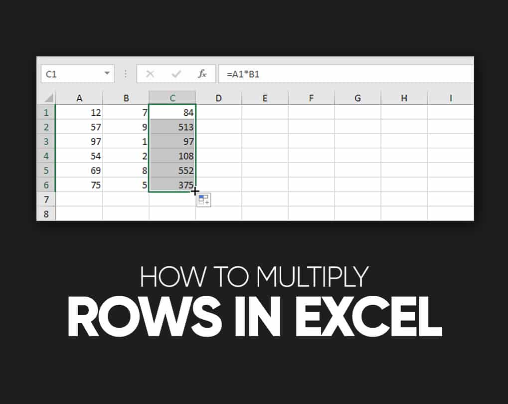
How to Multiply Rows in Excel
Multiplying rows in Excel is a less familiar task, but there is a simple solution for it too. To multiply two rows in MSExcel, do the following:
- Enter a multiplication formula in the first (leftmost) cell.
- In this example, we multiply values in row 1 by the values in row 2, beginning with column B. So our formula goes as follows: =B1*B2
- Choose the formula cell, and hover the mouse cursor over a little square at the lower right-hand corner until it changes to a thick black cross.
- Pull that black cross rightward over the cells where you need to copy the formula.
As with multiplying columns, the corresponding cell references in the formula change based on a relative position of rows and columns, multiplying a value in row 1 by a value in row 2 in each column.
How to Multiply in MSExcel – Multiply Function in Excel (PRODUCT)
If you want to multiply multiple cells or ranges, the fastest method would be using the PRODUCT function:
PRODUCT(number1, [number2], …)
Where number1, number2, etc. are numbers, cells, or areas that you need to multiply.
For instance, to multiply values in cells A2, B2, and C2, apply this formula:
=PRODUCT(A2:C2)
To multiply the figures in cells A2 through C2, and then multiply the outcome by 3, use this one:
=PRODUCT(A2:C2,3)
Multiply Numbers in Excel by Using the Product Formula
You can use the basic formula to cross multiply the numbers in MSexcel if you use the product formula to multiply up to 255 values at once.
- So, First, go to MS Excel and choose any blank cell. Then type an equal symbol, followed by the word PRODUCT. Next, add an opening addition.
- Multiply Individual Cells, type the names of the cells and divide them with commas without space.
- To Multiply a Series of Cells, type a colon between two cells’ names to specify that all cells within that range should be multiplied. For instance, “=PRODUCT(A2:A5)” point out that cells A2,A3, A4, and A5 should be multiplied.
- If you want to add a number to the equation, so enter a comma and then that number.
- When you complete entering the Values of your formula, then put a closing Parenthesis at last and hit the “Enter” button on your Keyboard. The equation answer will all show in the cell.
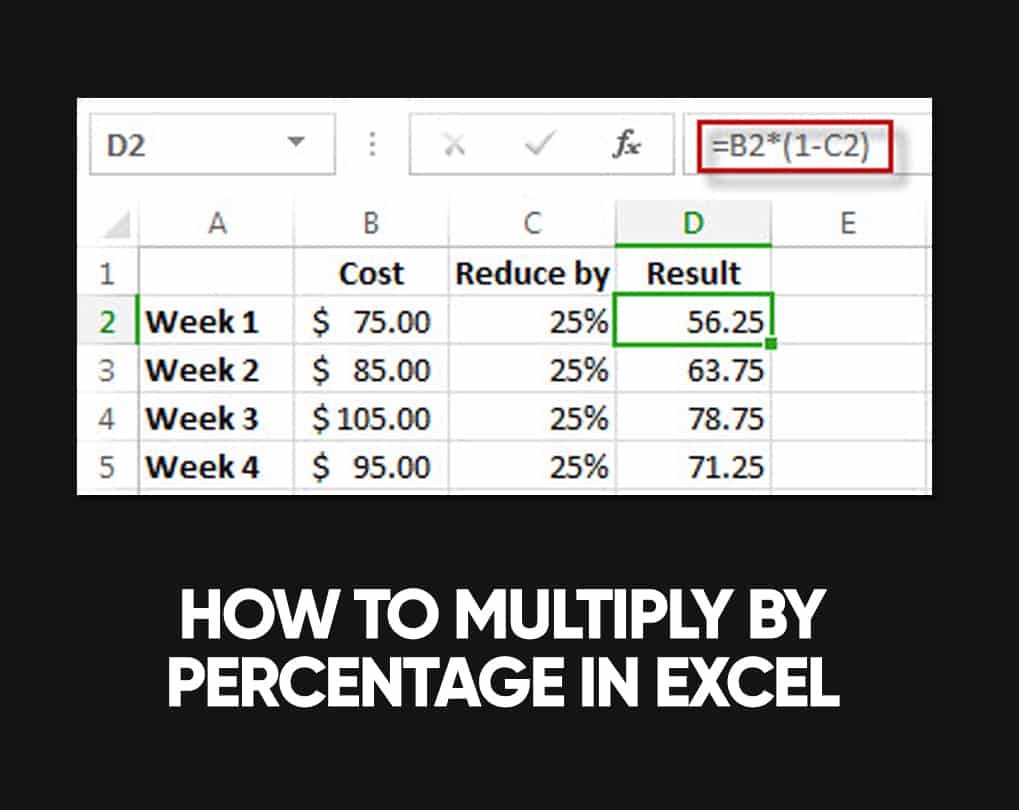
How to Multiply by Percentage in Excel
To multiply percentages in MSExcel, do a multiplication formula in this way: type the equals sign, followed by the number or cell, followed by the multiply sign (*), followed by a percentage.
In other terms, make a formula similar to these:
- To multiply a number by percentage: =50*10%
- To multiply a cell by percentage: =A1*10%
Rather than percentages, you can multiply by a similar decimal number. For example, knowing that 10 percent is ten parts of a hundred (0.1), use the following expression to multiply 50 by 10%: =50*0.1
How to Multiply a Column by a Number in the Excel
To multiply a column of numbers by the corresponding number, proceed with these steps:
- Insert the number to multiply by in some cell, say in A2.
- Type a multiplication formula for the topmost cell in the column.
- Considering the numbers to be multiplied are in column C, beginning in row 2. You set the following formula in D2:
- =C2*$A$2
- You must lock the column and row coordinates of the cell with the number to multiply by to prevent the reference from changing when you copy the formula to other cells. For this, type the $ symbol before the column letter and row number to make an absolute reference ($A$2). Or, click on the reference and press the F4 key to change it to complete.
- Double-click enough handle in the formula cell (D2) to copy the formula down the column. Done!
C2 (relative reference) changes to C3 when the formula is copied to row 3, while $A$2 (absolute reference) continues unchanged:
If the design of your worksheet does not provide an additional cell to accommodate the number, you can supply it directly in the formula, e.g., =C2*3
You can also apply the Paste Special > multiply feature to multiply a column by a constant number and get the results as values rather than formulas. Please check out this example for detailed instructions.
How to Multiply and Sum in Excel
When you require to multiply two columns or rows of numbers, and then add up the results of different calculations, use the SUMPRODUCT function to multiply cells and sum products.
Assuming you have prices in column B, quantity in column C, and calculate the total value of sales. In your math class, you’d multiply each Price/Qty. Pair individually and add up the sub-totals.
In Microsoft Excel, all these computations can be done with a single formula:
=SUMPRODUCT(B2:B5,C2:C5)
If you want, you can check the outcome with this calculation:
=(B2*C2)+(B3*C3)+(B4*C4)+(B5*C5)
And make assured the SUMPRODUCT formula multiplies and sums correctly:
Multiplication in Array Formulas
In case you want to multiply two columns of numbers and then perform further calculations with the results. Do multiplication within an array formula.
In the higher data set, another way to calculate the total value of sales is this:
=SUM(B2:B5*C2:C5)
This Excel Sum Multiply formula is equivalent to SUMPRODUCT and returns precisely the same result.
Taking the case further, let’s find an average sales. For this, use the AVERAGE function instead of SUM:
=AVERAGE(B2:B5*C2:C5)
To find the most extensive and smallest sale, use the MAX and MIN functions, respectively:
=MAX(B2:B5*C2:C5)
=MIN(B2:B5*C2:C5)
To complete an array formula correctly, be sure to press the Ctrl + Shift + Enter combination instead of entering a stroke. As quickly as you do this, Excel will enclose the formula in {curly braces}, indicating it’s an array formula.
Conclusion
Suppose you belong to any organization or company. In that case, this guide will be helpful for you because it includes all the multiplication methods and it means a lot to every organizational person. Multiplication in excel is not as difficult as you think. But if you want to do it quickly, you must memorize the formula to convert the complex method into an easy method. Let us know how much the excel sheet is helpful for you.
Maintenance Alert: Saturday, April 15th, 7:00pm-9:00pm CT. During this time, the shopping cart and information requests will be unavailable.
Categories: Formulas
Tags: Multiply Formula
While there is no “Excel multiply formula” there are multiple ways to multiply in Excel. For instance, do you use an asterisk (*) to multiply, but hit a brick wall when you apply other arithmetic operators? What about shortcuts for multiplying many numbers in one step?
Read on for three powerful ways to perform an Excel multiply formula.
1. Multiplication with *
To write a formula that multiplies two numbers, use the asterisk (*). To multiply 2 times 8, for example, type “=2*8”.
Use the same format to multiply the numbers in two cells: “=A1*A2” multiplies the values in cells A1 and A2.
You can mix and match the * with other arithmetic operators, such as addition (+), subtraction (-), division (/), and exponentiation (^). In these cases, remember that Excel carries out the operations in the order of PEMDAS: parentheses first, followed by exponents, multiplication, division, addition, and subtraction.
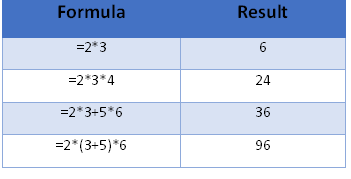
In the following formula “=2*3+5*6,” Excel performs the two multiplication operations first, obtaining 6+30, and add the products to reach 36.
What if you want to add 3+5 before performing the multiplication? Use parentheses. Excel will always evaluate anything in parentheses before resuming the remaining calculations following PEMDAS. In the case of “=3*(3+5)*6”, Excel adds 3 and 5 first, resulting in 8. Then it multiplies 3*8*6 and reaches 144.
If you have trouble remembering the order of PEMDAS, use the Aunt Sally mnemonic device: use the first letters of the sentence, “Please Excuse My Dear Aunt Sally.”
2. Multiplication with the PRODUCT Function
When you need to multiply several numbers, you might appreciate the shortcut formula PRODUCT, which multiplies all of the numbers that you include in the parentheses.
The arguments can be:
- Numbers or formulas separated by commas, such as:
=PRODUCT(3,5+2,8,3.14)
This is equivalent to =3*(5+2)*8*3.14.
- Cell references separated by commas, such as:
=PRODUCT(A3,C3,D3,F3).
This is equivalent to =A3*C3*D3*F3.
- A range of cells containing numbers, or multiple ranges separated by commas, such as:
=PRODUCT(F3:F25),
which is equivalent to =F3*F4*F5*(and so on, all the way up to)*F25, or:
=PRODUCT(F3:F25,H3:H25).
- Any combination of numbers, formulas, cell references, and range references.
In each case, Excel multiplies all the numbers to find the product. If a cell in the range is empty or contains text, Excel leaves that cell’s value out of the calculation. If a cell in the range is zero, the product will be zero.
3. Multiplication of Ranges with the SUMPRODUCT Function
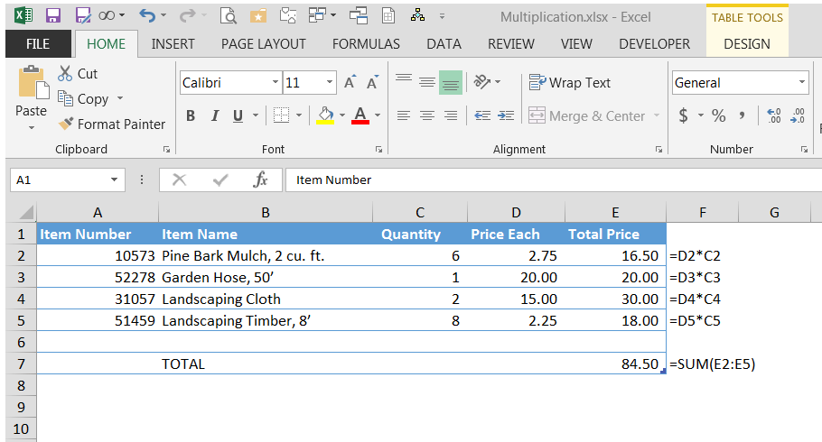
Consider the following invoice. The formula in Column E (with the formula shown to the right of the table) multiplies quantity by the price each to reach an extended price. The total in cell E7 sums up the extended prices.
But what if you don’t want the extended prices to show as separate calculations? What if you want to do it all in one step?
Try the SUMPRODUCT function, which multiplies the cells in two ranges and sums the results.
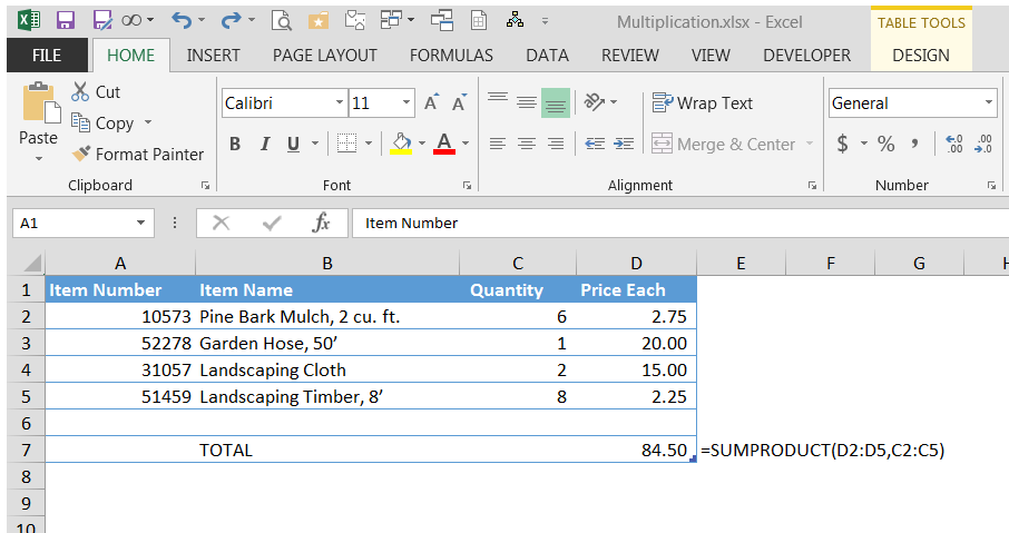
SUMPRODUCT(D2:D5,C2:C5) multiplies D2*C2, D3*C3, etc., and sums the results. Note that the result, 84.50, is the same as the previous example.
This function is invaluable for calculating weighted averages, such as classroom grades or prices based on variable state tax, in which you multiply a range of values by a range containing the weights.
Next Steps
These are but three of the methods to multiply numbers in Excel formulas. When you’ve mastered them, try the PRODUCTIF formula, which multiplies all numbers in a range if a condition is met.
Until then, try mixing and matching the multiplication formulas, using any combination along with other arithmetic functions, to create complex mathematical models.
PRYOR+ 7-DAYS OF FREE TRAINING
Courses in Customer Service, Excel, HR, Leadership,
OSHA and more. No credit card. No commitment. Individuals and teams.