
There are many functions in order to find the average in Excel (although it does not matter what kind of value it is: numerical, textual, percentage or other). And each of them has its own peculiarities and advantages. After all, certain conditions can be put in this task.
For example, the average in Excel is counting using statistical functions. You can also manually enter your own formula. Consider the various options.
How to find the arithmetic mean?
It is necessary to add all the numbers in the set and divide the sum by the number in order to find the arithmetic mean. For example, the student’s marks in computer science: 3, 4, 3, 5, 5. The average rating is 4 for a quarter. We found the arithmetic mean using the formula: =(3 + 4 + 3 + 5 + 5) / 5.
How can you quickly do this with Excel functions? Take for example a number of random numbers in a row:

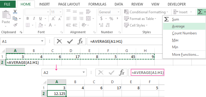
- We put the cursor in cell A2 (under a set of numbers). In the menu – «HOME»-«Editing»-«AutoSum»-«Average» button. A formula appears after clicking in the active cell. Select the range: A1: H1 and press ENTER.
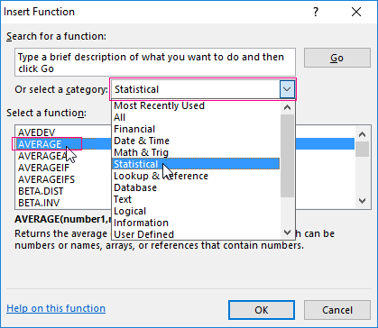
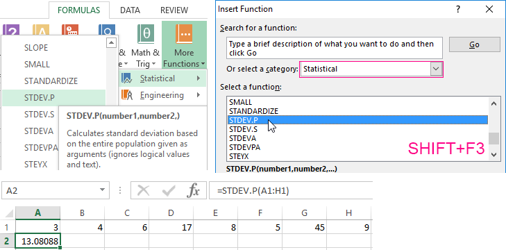
- The second method is based on the same principle of finding the arithmetic mean. But we will call the function AVERAGE differently. Using the function wizard (use fx button or key combination SHIFT + F3).
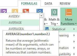
- The third way to call the AVERAGE function from the panel: «FORMULAS»-«More Function»-«Statistical»-«AVERAGE».
Or you can make cell to be active and just manually enter the formula: =AVERAGE(A1:A8).
Now let’s see what the AVERAGE function be able to:
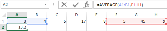
Let us find the arithmetic mean of the first two and three last numbers. Formula: =AVERAGE(A1:B1,F1:H1).
Average value by condition
A numerical criterion or a textual criterion can be the condition for finding the arithmetic mean. We will use the function: = AVERAGEIF().
Find the arithmetic mean for numbers that are greater or equal to 10.
Function:
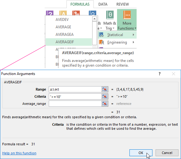
The result of using the function «AVERAGEIF» by the condition «>=10» is next:
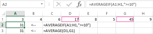
The third argument «Averaging Range» is omitted. Firstly, it is not necessary. Secondly, the range analyzed by the program contains ONLY numeric values. In the cells specified in the first argument, the search will be performed according to the condition specified in the second argument.
Attention! You can specify the search criteria in the cell. And in the formula make a reference to it.
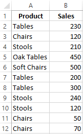
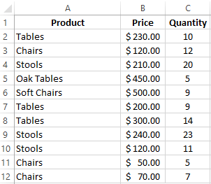
Let’s find the average value of numbers by the text criterion. For example, the average sales of goods «Tables».
The function will look like this:
Range is a column with the names of goods. Search criteria is a link to a cell with the word «Tables» (you can insert the word «Tables» instead of the A7 link). The averaging range is the cells from which data will be taken to calculate the arithmetic mean.
We get the following value as a result of calculating using the function:
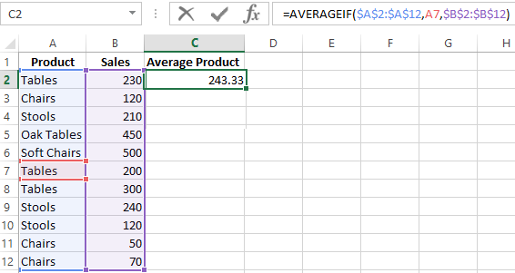
Attention! It is mandatory to point the averaging range for the text criterion (condition).
How to calculate the weighted average price in Excel?
How to calculate the average percentage in Excel? For this purpose, the SUMPRODUCTS and SUM functions are suitable. Table for an example:
How did we know the weighted average price?
Formula:
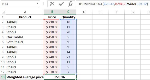
Using the formula =SUMPRODUCT() we learn the total revenue after the realization of the entire quantity of goods. And the =SUM() function sums the goods quantity. We found a weighted average price having divided the total revenue from the sale of goods by the total number of units of the goods. This indicator takes into account the «weight» of each price and its share in the total mass of values.
The standard deviation: the formula in Excel
There is a standard deviation in the entire population and in the sampling. In the first case, this is the square root of the general variance. In the second, this is a square root of the sampling variance.
A dispersion formula is compiled to calculate this statistical indicator. The square root is extracted from it. But in Excel, there is a ready-made function for finding the root-mean-square deviation.
The root-mean-square deviation is related to the scope of the initial data. This is not enough for a figurative representation of the variation of the analyzed range. The coefficient of variation is calculated to obtain the relative level of the data variability.
standard deviation / arithmetic mean
The formula in Excel is as follows:
STDEV.P (range of values) / AVERAGE (range of values).
The coefficient of variation is considered as a percentage. Therefore, set the percentage format in the cell set.
How to Find Mean in Excel (Table of Content)
- Introduction to Mean in Excel
- Example of Mean in Excel
Introduction to Mean in Excel
The average function is used to calculate the Arithmetic Mean of the given input. It is used to do sum of all arguments and divide it by the count of arguments where the half set of the number will be smaller than the mean, and the remaining set will be greater than the mean. It will return the arithmetic mean of the number based on provided input. It is an in-built Statistical function. A user can give 255 input arguments in the function.
As an example, suppose there is 4 number 5,10,15,20 if a user wants to calculate the mean of the numbers then it will return 12.5 as the result of =AVERAGE (5, 10, 15, 20).
The formula of Mean: It is used to return the mean of the provided number where a half set of the number will be smaller than the number, and the remaining set will be greater than the mean.
The argument of the Function:
- number1: It is a mandatory argument in which functions will take to calculate the mean.
- [number2]: It is an optional argument in the function.
Examples on How to Find Mean in Excel
Here are some examples of how to find mean in excel with the steps and the calculation
You can download this How to Find Mean Excel Template here – How to Find Mean Excel Template
Example #1 – How to Calculate the Basic Mean in Excel
Let’s assume there is a user who wants to perform the calculation for all numbers in Excel. Let’s see how we can do this with the average function.
Step 1: Open MS Excel from the start menu >> Go to Sheet1, where the user has kept the data.
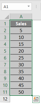
Step 2: Now create headers for Mean where we will calculate the mean of the numbers.
![]()
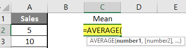
Step 3: Now calculate the mean of the given number by average function>> use the equal sign to calculate >> Write in cell C2 and use average>> “=AVERAGE (“
Step 3: Now, it will ask for a number1, which is given in column A >> there are 2 methods to provide input either a user can give one by one or just give the range of data >> select data set from A2 to A11 >> write in cell C2 and use average>> “=AVERAGE (A2: A11) “
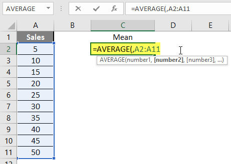
Step 4: Now press the enter key >> Mean will be calculated.
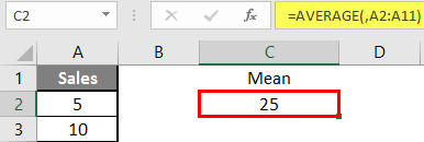
Summary of Example 1: As the user wants to perform the mean calculation for all numbers in MS Excel. Easley everything calculated in the above excel example, and the Mean is 27.5 for sales.
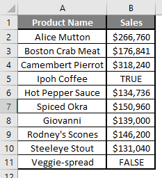
Example #2 – How to Calculate Mean if Text Value Exists in the Data Set
Let’s calculate the Mean if there is some text value in the Excel data set. Let’s assume a user wants to perform the calculation for some sales data set in Excel. But there is some text value also there. So, he wants to use count for all, either its text or number. Let’s see how we can do this with the AVERAGE function. Because in the normal AVERAGE function, it will exclude the text value count.
Step 1: Open MS Excel from the start menu >> Go to Sheet2, where the user has kept the data.
Step 2: Now create headers for Mean where we will calculate the mean of the numbers.
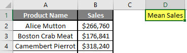
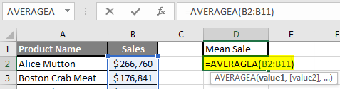
Step 3: Now calculate the mean of the given number by average function>> use the equal sign to calculate >> Write in cell D2 and use AVERAGEA>> “=AVERAGEA (“
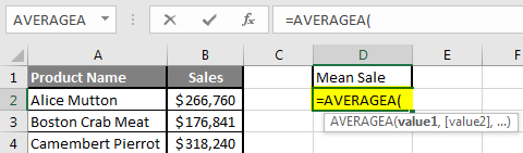
Step 4: Now, it will ask for a number1, which is given in column B >> there is two open to provide input either a user can give one by one or just give the range of data >> select data set from B2 to B11 >> write in D2 Cell and use average>> “=AVERAGEA (D2: D11) “
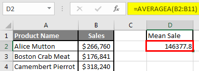
Step 5: Now click on the enter button >> Mean will be calculated.
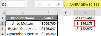
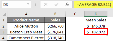
Step 6: Just to compare the AVERAGEA and AVERAGE, in normal average, it will exclude the count for text value so mean will high than the AVERAGE MEAN.
Summary of Example 2: As the user wants to perform the mean calculation for all number in MS Excel. Easley, everything calculated in the above excel example and the Mean is $146377.80 for sales.
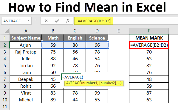
Example #3 – How to Calculate Mean for Different Set of Data
Let’s assume a user wants to perform the calculation for some student’s mark data set in MS Excel. There are ten student marks for Math, English, and Science out of 100. Let’s see How to Find Mean in Excel with the AVERAGE function.
Step 1: Open the MS Excel from the start menu >> Go to Sheet3, where the user kept the data.
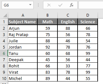
Step 2: Now create headers for Mean where we will calculate the mean of the numbers.
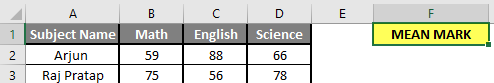
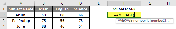
Step 3: Now calculate the mean of the given number by average function>> use the equal sign to calculate >> Write in F2 Cell and use AVERAGE >> “=AVERAGE (“
Step 3: Now, it will ask for number1 which is given in B, C, and D column >> there is two open to provide input either a user can give one by one or just give the range of data >> Select data set from B2 to D2 >> Write in F2 Cell and use average >> “=AVERAGE (B2: D2) “
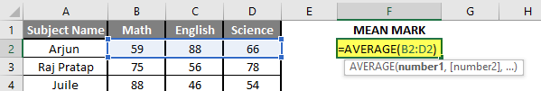
Step 4: Now click on the enter button >> Mean will be calculated.
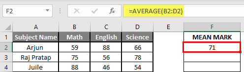
Step 5: Now click on the F2 cell and drag and apply to another cell in the F column.
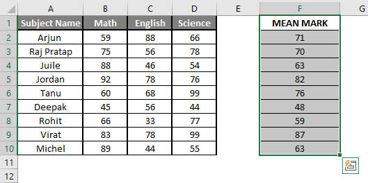
Summary of Example 3: As the user wants to perform the mean calculation for all number in MS Excel. Easley, everything calculated in the above excel example and the Mean is available in the F column.
Things to Remember About How to Find Mean in Excel
- Microsoft Excel’s AVERAGE function used to calculate the Arithmetic Mean of the given input. A user can give 255 input arguments in the function.
- Half the set of a number will be smaller than the mean, and the remaining set will be greater than the mean.
- If a user calculating the normal average, it will exclude the count for a text value, so AVERAGE Mean will bigger than the AVERAGE MEAN.
- Arguments can be number, name, range or cell references that should contain a number.
- If a user wants to calculate the mean with some condition, then use AVERAGEIF or AVERAGEIFS.
Recommended Articles
This is a guide to How to Find Mean in Excel. Here we discuss How to Find Mean along with examples and a downloadable excel template. You may also look at the following articles to learn more –
- FIND Function in Excel
- Excel Find
- Excel Average Formula
- Excel AVERAGE Function
Calculating the mean of numbers is one of staples of statistical analysis processes. In this article, we’re going to show you how to calculate mean in Excel using the AVERAGE formula.
Syntax
=AVERAGE( array of numbers )
Steps
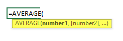
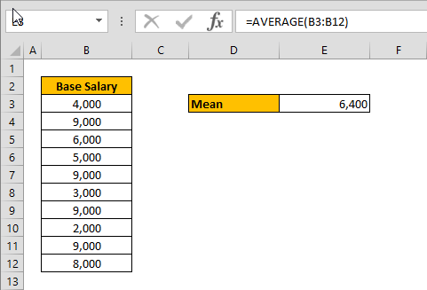
- Begin by creating the formula =AVERAGE(
- Select your data range that contains the values (i.e. B3:B12)
- Finish the formula with ) and press the Enter key.
How to find the mean in Excel
The mean or the statistical mean is essentially means average value and can be calculated by adding data points in a setand then dividing the total, by the number of points. Excel’s AVERAGE function does exactly this: sum all the values and divides the total by the count of numbers.
The AVERAGE function can also be configured to ignore empty cells and cells that do not include any numbers. If you want to include empty or invalid values in calculations as zeroes, use the AVERAGEA function. The AVERAGEA function works exactly the same with the AVERAGE.
=AVERAGEA( array of numbers )
For more information about AVERAGE formula please see our related article.
You can use the following formulas to find the mean, median, and mode of a dataset in Excel:
=AVERAGE(A1:A10)

=MEDIAN(A1:A10)

=MODE.MULT(A1:A10)
It’s worth noting that each of these formulas will simply ignore non-numeric or blank values when calculating these metrics for a range of cells in Excel.
The following examples shows how to use these formulas in practice with the following dataset:

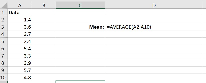
Example: Finding the Mean in Excel
The mean represents the average value in a dataset.
The following screenshot shows how to calculate the mean of a dataset in Excel:

The mean turns out to be 19.11.
Example: Finding the Median in Excel
The median represents the middle value in a dataset, when all of the values are arranged from smallest to largest.
The following screenshot shows how to calculate the median of a dataset in Excel:

The median turns out to be 20.
Example: Finding the Mode in Excel
The mode represents the value that occurs most often in a dataset. Note that a dataset can have no mode, one mode, or multiple modes.
The following screenshot shows how to calculate the mode(s) of a dataset in Excel:

The modes turn out to be 7 and 25. Each of these values appears twice in the dataset, which is more often than any other value occurs.
Note: If you use the =MODE() function instead, it will only return the first mode. For this dataset, only the value 7 would be returned. For this reason, it’s always a good idea to use the =MODE.MULT() function in case there happens to be more than one mode in the dataset.
Additional Resources
How to Calculate the Interquartile Range (IQR) in Excel
How to Calculate the Midrange in Excel
How to Calculate Standard Deviation in Excel
In this guide, I will show you how to calculate the mean (average), standard deviation (SD) and standard error of the mean (SEM) by using Microsoft Excel.
Calculating the mean and standard deviation in Excel is pretty easy. These have built-in functions already available.
Calculating the standard error in Excel, however, is a bit trickier. There is no formula within Excel to use for this, so I will show you how to calculate this manually.
How to calculate the mean value in Excel
The mean, or average, is the sum of the values, divided by the number of values in the group.
To calculate the mean, follow the steps below.
1. Click on an empty cell where you want the mean value to be.
2. Enter the following formula.
=AVERAGE(number1:number2)
Then change the following:
- Number1 – the cell that is at the start of the list of values
- Number2 – the cell that is at the end of the list of values
You can simply click and drag on the values within Excel instead of typing the cell names.
3. Then press the ‘enter’ button to calculate the mean value.
How to calculate the standard deviation in Excel
The standard deviation (SD) is a value to indicate the spread of values around the mean value.
To calculate the SD in Excel, follow the steps below.
1 Click on an empty cell where you want the SD to be.
2. Enter the following formula
=STDEV(number1:number2)
Then, as with the mean calculation, change the following:
- Number1 – the cell that is at the start of the list of values
- Number2 – the cell that is at the end of the list of values
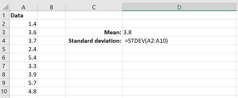
3. Then press the ‘enter’ button to calculate the SD.
How to calculate the standard error in Excel
The standard error (SE), or standard error of the mean (SEM), is a value that corresponds to the standard deviation of a sampling distribution, relative to the mean value.
The formula for the SE is the SD divided by the square root of the number of values n the data set (n).
To calculate the SE in Excel, follow the steps below.
1. Click on an empty cell where you want the SE to be.
2. Enter the following into the cell:
=STDEV(number1:number2)/SQRT(COUNT(number1:number2))
Change the following throughout:
- Number1 – the cell that is at the start of the list of values
- Number2 – the cell that is at the end of the list of values
It is worth noting that instead of using the COUNT function, you can simply type in the number of values in the data set. In this example, this would be 9.
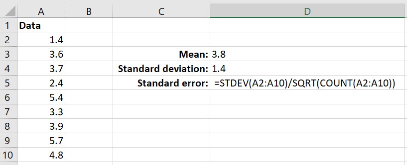
3. Then press the ‘enter’ button to calculate the SE.
Conclusion
In this tutorial, I have described how to calculate the mean, SD and SE by using Microsoft Excel.
Microsoft Excel version used: Office 365 ProPlus