Formula for excel cell color

You can use a formula in conjunction with an Event Macro. Pick a cell, say B2 and enter the formula:

=IF(A1>10,"black","green")

Then format B2 Custom ;;;
This will hide the displayed text.
Then place the following event macro in the worksheet code area:

Private Sub Worksheet_Calculate()
Application.EnableEvents = False
    With Range("B2")
        If .Value = "green" Then
            .Interior.Color = RGB(0, 255, 0)
        Else
            .Interior.Color = RGB(0, 0, 0)
        End If
    End With
Application.EnableEvents = True
End Sub

The macro will run every time the worksheet is re-calculated. It will exame the text in B2 (even though the text is not visible) and adjust the backgound color accordingly.

Because it is worksheet code, it is very easy to install and automatic to use:

1. right-click the tab name near the bottom of the Excel window
2. select View Code — this brings up a VBE window
3. paste the stuff in and close the VBE window

If you have any concerns, first try it on a trial worksheet.

If you save the workbook, the macro will be saved with it.
If you are using a version of Excel later then 2003, you must save
the file as .xlsm rather than .xlsx

To remove the macro:

1. bring up the VBE windows as above
2. clear the code out
3. close the VBE window

To learn more about macros in general, see:

http://www.mvps.org/dmcritchie/excel/getstarted.htm

and

http://msdn.microsoft.com/en-us/library/ee814735(v=office.14).aspx

To learn more about Event Macros (worksheet code), see:

http://www.mvps.org/dmcritchie/excel/event.htm

Macros must be enabled for this to work!

@Radish_G 

You may use the following User Defined Function to get the Color Index or RGB value of the cell color.

Place the following function on a Standard Module like Module1…

Function getColor(Rng As Range, ByVal ColorFormat As String) As Variant
    Dim ColorValue As Variant
    ColorValue = Cells(Rng.Row, Rng.Column).Interior.Color
    Select Case LCase(ColorFormat)
        Case "index"
            getColor = Rng.Interior.ColorIndex
        Case "rgb"
            getColor = (ColorValue Mod 256) & ", " & ((ColorValue  256) Mod 256) & ", " & (ColorValue  65536)
        Case Else
            getColor = "Only use 'Index' or 'RGB' as second argument!"
    End Select
End Function

And then assuming you want to check the color index or the RGB of the cell A2, try the UDF on the worksheet like below…

To get Color Index:

=getcolor(A2,"index")

To get RGB:

=getcolor(A2,"rgb")

Let’s say that one of our tasks is to entering of the information about: did the ordering to a customer in the current month. Then on the basis of the information you need to select the cell in color according to the condition: which from customers have not made any orders for the past 3 months. For these customers you will need to re-send the offer.

Of course it’s the task for Excel. The program should automatically find such counterparties and, accordingly, to color ones. For these conditions we will use to the conditional formatting.



The filling cells with dates automatically

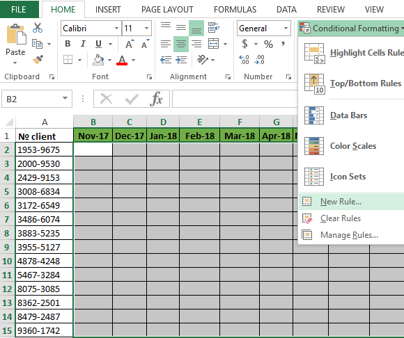
At first, you need to prepare to the structure for filling the register. First of all, let’s consider to the ready example of the automated register, which is depicted in the picture below. Today date 07.07.2018:

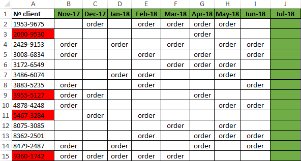
The user to need only to specify, if the customer have made an order in the current month, in the corresponding cell you should enter the text value of «order». The main condition for the allocation: if for 3 months the contractor did not make any order, his number is automatically highlighted in red.

Presented this decision should automate some work processes and to simplify to the visual data analysis.

The automatic filling of the cells with the relevant dates

At first, for the register with numbers of customers we will create to the column headers with green and up to date for months that will automatically display to the periods of time. To do this, in the cell B1 you need to enter the following formula:

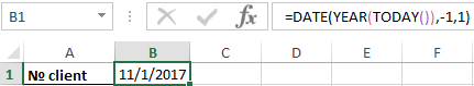
How does the formula work for automatically generating of the outgoing months?

In the picture, the formula returns the period of time passing since the date of writing this article: 17.09.2017. In the first argument in the function DATE is the nested formula that always returns the current year to today’s date thanks to the functions: YEAR and TODAY. In the second argument is the month number (-1). The negative number means that we are interested in what it was a month last time. The example of the conditions for the second argument with the value:

• 1 means the first month (January) in the year that is specified in the first argument;
• 0 – it is 1 month ago;
• -1 – there is 2 months ago from the beginning of the current year (i.e. 01.10.2016).

The last argument-is the day number of the month, which is specified in the second argument. As a result, the DATE function collects all parameters into a single value and the formula returns to the corresponding date.

Next, go to the cell C1 and type the following formula:

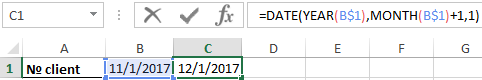
As you can see now the DATE function uses the value from the cell B1 and increases to the month number by 1 in relation to the previous cell. As the result is the 1 – the number of the following month.

Now you need to copy this formula from the cell C1 in the rest of the column headings in the range D1:AY1.

To highlight to the cell range B1:AY1 and select to the tool: «HOME»-«Cells»-«Format Cells» or just to press CTRL+1. In the dialog box that appears, in the tab «Number» in the section «Category» you need to select the option «Custom». In the «Type:» to enter the value: MMM. YY (required the letters in upper register). Because of this, we will get to the cropped display of the date values in the headers of the register, what simplifies to the visual analysis and make it more comfortable due to better readability.

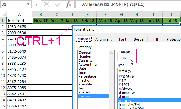
Please note! At the onset of the month of January (D1), the formula automatically changes in the date to the year in the next one.



How to select the column by color in Excel under the terms

Now you need to highlight to the cell by color which respect of the current month. Because of this, we can easily find the column in which you need to enter the actual data for this month. To do this:

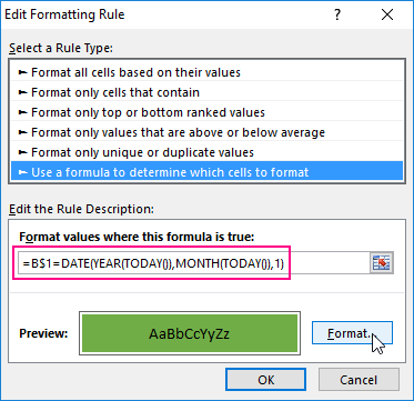
1. To select the range of the cells B2:AY15 and select the tool: «HOME» -«Styles» -«Conditional Formatting»-«New Rule». And in the appeared window «New Formatting Rule» you need to select the option: «Use a formula to determine which cells to format»



2. In the input field to enter the formula:



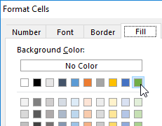
3. Click «Format» and indicate on the tab «Fill» in what color (for example green) will be the selected cells of the current month. Then on all Windows for confirmation to click «OK».

The column under the appropriate heading of the register is automatically highlighted in green accordingly to our terms and conditions:

How does the formula highlight of the column color on a condition work?

Due to the fact that before the creation of the conditional formatting rule we have covered all the table data for inputting data of register, the formatting will be active for each cell in the range B2:AY15. The mixed reference in the formula B$1 (absolute address only for rows, but for columns it is relative) determines that the formula will always to refer to the first row of each column.

Automatic highlighting of the column in the condition of the current month

The main condition for the fill by color of the cells: if the range B1:AY1 is the same date that the first day of the current month, then the cells in a column change its colors by specified in conditional formatting.

Please note! In this formula, for the last argument of the function DATE is shown 1, in the same way as for formulas in determining the dates for the column headings of the register.

In our case, is the green filling of the cells. If we open our register in next month, that it has the corresponding column is highlighted in green regardless of the current day.

The table is formatted, now we are filling it with the text value of the «order» in a mixed order of clients for current and past months.

How to highlight the cells in red color according to the condition

Now we need to highlight in red to the cells with the numbers of clients who for 3 months have not made any order. To do this:

1. Select the range of the cells A2:A15 (that is, the list of the customer numbers) and select to the tool: «HOME»-«Styles»-«Conditional formatting»-«Create rule». And in the window that appeared «Create a formatting rule» to select the option: «Use the formula for determining which cells to format».
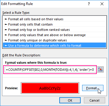
2. This time in the input box to enter the formula:



3. To click «Format» and specify the red color on the tab «Fill». Then on all Windows click «OK».
4. Fill the cells with the text value of «order» as in the picture and look at the result:

The numbers of customers are highlighted in red, if in the row has no have the value «order» in the last three cells for the current month (inclusively).

The analysis of the formula for the highlighting of cells according to the condition

Firstly, we will do by the middle part of our formula. The SHIFT function returns a range reference shifted relative to the basic range of the certain number of rows and columns. The returned reference can be a single cell or a range of cells. Optionally, you can define to the number of returned rows and columns. In our example, the function returns the reference to the cell range for the last 3 months.

The important part for our terms of highlighting in color – is belong to the first argument of the SHIFT function. It determines from which month to start the offset. In this example, there is the cell D2, that is, the beginning of the year – January. Of course for the rest of the cells in the column the row number for the base of the cell will correspond to the line number in what it is located. The following 2 arguments of the SHIFT function to determine how many rows and columns should be done offset. Since the calculations for each customer will carry in the same line, the offset value for the rows we specified is -0.

At the same time for the calculating the value of the third argument (the offset by the columns) we use to the nested formula MONTH(TODAY()), which in accordance with the terms returns to the number of the current month in the current year. From the calculated formula of the month as a number subtract the number 4, that is, in cases November we get the offset by 8 columns. And, for example, for June – there are on 2 columns only.

The last two arguments for the SHIFT function, determine the height (in the number of rows) and width (in the number of columns) of the returned range. In our example, there is the area of the cell with height on 1 row and with width on 4 columns. This range covers to the columns of 3 previous months and the current month.

The first function in the COUNTIF formula checks the condition: how many times in the returned range using the SHIFT function, we can found to the text value «order». If the function returns the value of 0, it means from the client with this number for 3 months there was not any order. And in accordance with our terms and conditions, the cell with number of this client is shown in red fill color.

If we want to register to data for customers, Excel is ideally suited for this purpose. You can easily record in the appropriate categories to the number of ordered goods, as well as the date of implementation of transaction. The problem gradually starts with arising of the data growth.

Download example automatic highlight cells by color.

If so many of them that we need to spend a few minutes looking for a specific position of the register and analysis of the information entered. In this case, it is necessary to add in the table to the register of mechanisms to automate some workflows of the user. And so we did.