
Excel for Microsoft 365 Excel for Microsoft 365 for Mac Excel for the web Excel 2021 Excel 2021 for Mac Excel 2019 Excel 2019 for Mac Excel 2016 Excel 2016 for Mac Excel 2013 Excel for iPad Excel for iPhone Excel for Android tablets Excel 2010 Excel 2007 Excel for Mac 2011 Excel for Android phones Excel Starter 2010 More…Less
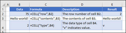
The CELL function returns information about the formatting, location, or contents of a cell. For example, if you want to verify that a cell contains a numeric value instead of text before you perform a calculation on it, you can use the following formula:
=IF(CELL(«type»,A1)=»v»,A1*2,0)
This formula calculates A1*2 only if cell A1 contains a numeric value, and returns 0 if A1 contains text or is blank.
Note: Formulas that use CELL have language-specific argument values and will return errors if calculated using a different language version of Excel. For example, if you create a formula containing CELL while using the Czech version of Excel, that formula will return an error if the workbook is opened using the French version. If it is important for others to open your workbook using different language versions of Excel, consider either using alternative functions or allowing others to save local copies in which they revise the CELL arguments to match their language.
Syntax
CELL(info_type, [reference])
The CELL function syntax has the following arguments:
|
Argument |
Description |
|---|---|
|
info_type Required |
A text value that specifies what type of cell information you want to return. The following list shows the possible values of the Info_type argument and the corresponding results. |
|
reference Optional |
The cell that you want information about. If omitted, the information specified in the info_type argument is returned for cell selected at the time of calculation. If the reference argument is a range of cells, the CELL function returns the information for active cell in the selected range. Important: Although technically reference is optional, including it in your formula is encouraged, unless you understand the effect its absence has on your formula result and want that effect in place. Omitting the reference argument does not reliably produce information about a specific cell, for the following reasons:
|
info_type values
The following list describes the text values that can be used for the info_type argument. These values must be entered in the CELL function with quotes (» «).
|
info_type |
Returns |
|---|---|
|
«address» |
Reference of the first cell in reference, as text. |
|
«col» |
Column number of the cell in reference. |
|
«color» |
The value 1 if the cell is formatted in color for negative values; otherwise returns 0 (zero). Note: This value is not supported in Excel for the web, Excel Mobile, and Excel Starter. |
|
«contents» |
Value of the upper-left cell in reference; not a formula. |
|
«filename» |
Filename (including full path) of the file that contains reference, as text. Returns empty text («») if the worksheet that contains reference has not yet been saved. Note: This value is not supported in Excel for the web, Excel Mobile, and Excel Starter. |
|
«format» |
Text value corresponding to the number format of the cell. The text values for the various formats are shown in the following table. Returns «-» at the end of the text value if the cell is formatted in color for negative values. Returns «()» at the end of the text value if the cell is formatted with parentheses for positive or all values. Note: This value is not supported in Excel for the web, Excel Mobile, and Excel Starter. |
|
«parentheses» |
The value 1 if the cell is formatted with parentheses for positive or all values; otherwise returns 0. Note: This value is not supported in Excel for the web, Excel Mobile, and Excel Starter. |
|
«prefix» |
Text value corresponding to the «label prefix» of the cell. Returns single quotation mark (‘) if the cell contains left-aligned text, double quotation mark («) if the cell contains right-aligned text, caret (^) if the cell contains centered text, backslash () if the cell contains fill-aligned text, and empty text («») if the cell contains anything else. Note: This value is not supported in Excel for the web, Excel Mobile, and Excel Starter. |
|
«protect» |
The value 0 if the cell is not locked; otherwise returns 1 if the cell is locked. Note: This value is not supported in Excel for the web, Excel Mobile, and Excel Starter. |
|
«row» |
Row number of the cell in reference. |
|
«type» |
Text value corresponding to the type of data in the cell. Returns «b» for blank if the cell is empty, «l» for label if the cell contains a text constant, and «v» for value if the cell contains anything else. |
|
«width» |
Returns an array with 2 items. The 1st item in the array is the column width of the cell, rounded off to an integer. Each unit of column width is equal to the width of one character in the default font size. The 2nd item in the array is a Boolean value, the value is TRUE if the column width is the default or FALSE if the width has been explicitly set by the user. Note: This value is not supported in Excel for the web, Excel Mobile, and Excel Starter. |
CELL format codes
The following list describes the text values that the CELL function returns when the Info_type argument is «format» and the reference argument is a cell that is formatted with a built-in number format.
|
If the Excel format is |
The CELL function returns |
|---|---|
|
General |
«G» |
|
0 |
«F0» |
|
#,##0 |
«,0» |
|
0.00 |
«F2» |
|
#,##0.00 |
«,2» |
|
$#,##0_);($#,##0) |
«C0» |
|
$#,##0_);[Red]($#,##0) |
«C0-« |
|
$#,##0.00_);($#,##0.00) |
«C2» |
|
$#,##0.00_);[Red]($#,##0.00) |
«C2-« |
|
0% |
«P0» |
|
0.00% |
«P2» |
|
0.00E+00 |
«S2» |
|
# ?/? or # ??/?? |
«G» |
|
m/d/yy or m/d/yy h:mm or mm/dd/yy |
«D4» |
|
d-mmm-yy or dd-mmm-yy |
«D1» |
|
d-mmm or dd-mmm |
«D2» |
|
mmm-yy |
«D3» |
|
mm/dd |
«D5» |
|
h:mm AM/PM |
«D7» |
|
h:mm:ss AM/PM |
«D6» |
|
h:mm |
«D9» |
|
h:mm:ss |
«D8» |
Note: If the info_type argument in the CELL function is «format» and you later apply a different format to the referenced cell, you must recalculate the worksheet (press F9) to update the results of the CELL function.
Examples
Need more help?
You can always ask an expert in the Excel Tech Community or get support in the Answers community.
See Also
Change the format of a cell
Create or change a cell reference
ADDRESS function
Add, change, find or clear conditional formatting in a cell
Need more help?
Return to Excel Formulas List
Download Example Workbook
Download the example workbook
This tutorial will demonstrate how to use a cell value in a formula in Excel and Google Sheets.
Cell Value as a Cell Reference
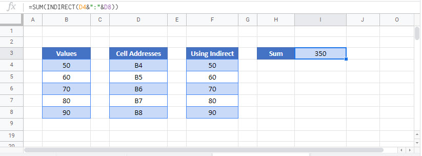
The INDIRECT Function is useful when you want to convert a text string in a cell into a valid cell reference, be it the cell address or a range name.
=INDIRECT(D4)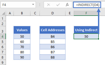
The INDIRECT Function will look at the text string in cell D4 which in this case is B4 – it will then use the text string as a valid cell reference and return the value that is contained in B4 – in this instance, 50.
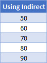
If you copy the formula down, the D4 will change to D5, D6 etc, and the correct value from column B will be returned.
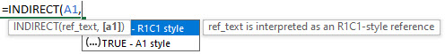
The Syntax of the INDIRECT Function is:
=INDIRECT(reference, reference style)The reference style can be either R1C1 style or can be the more familiar A1 style. If you omit this argument, the A1 style is assumed.
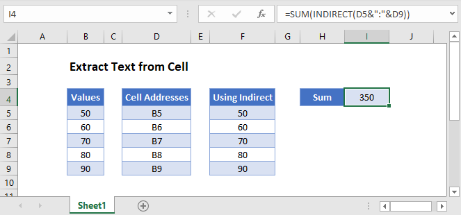
SUM Function With the INDIRECT Function
We can also use the INDIRECT function with the SUM Function to add up the values in column B by using the text strings in column D.
Click in H4 and type the following formula.
=SUM(INDIRECT(D4&":"&D8))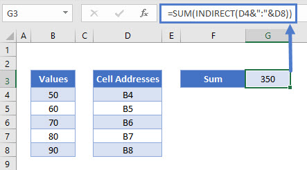
INDIRECT Function With Range Names in Excel
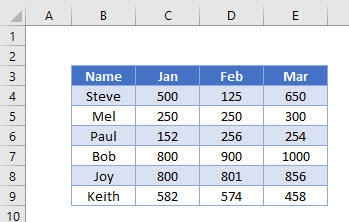
Now let’s look at an example of using the INDIRECT Function with Named Ranges.
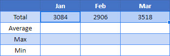
Consider the following worksheet where the sales figures are shown for a period of 3 months for several Sales Reps.
- Select the Range B3:E9.
- In the Ribbon, select Formulas > Create from Selection.
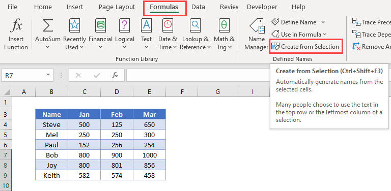
- Make sure that the Top row and the Left Column check boxes are ticked and click OK.
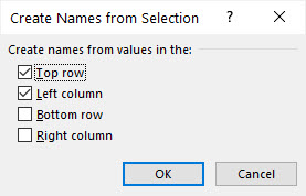
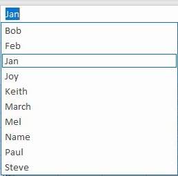
- Excel will now have created range names based on your selection.
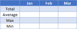
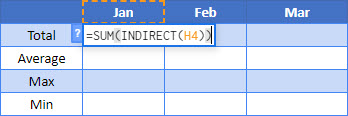
- Click in H4 and set up a table as shown below.
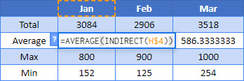
- In I4, type the following formula:
=SUM(INDIRECT(I3)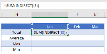
- Press Enter to complete the formula.
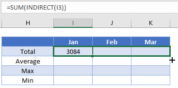
- Drag the formula across to column K.
- The formula will change from picking up I3 to picking up J3 (the Feb range name) and then K3 (the March range name).
- Repeat the process for the AVERAGE, MAX and MIN functions.
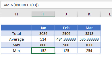
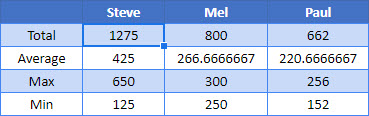
- We can then amend the names in row 3 to get the totals for 3 of the sales reps. The formulas will automatically pick up the correct values due to the INDIRECT
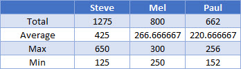
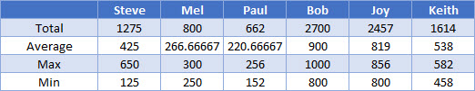
- Type in the name of the remaining reps in the adjacent column and drag the formulas across to get their sales figures.
Cell Value as a Cell Reference in Google Sheets
Using the INDIRECT Function in Google sheets works the same way as it does in Excel.
INDIRECT Function with Range Names in Google Sheets
Named Ranges work similar to Excel in Google Sheets.
- In the Menu, select Data>Named Ranges.
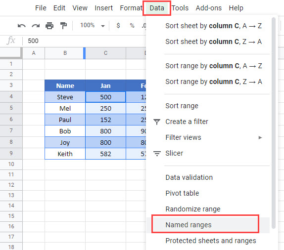
- Type in the name or the range, and then select the range.
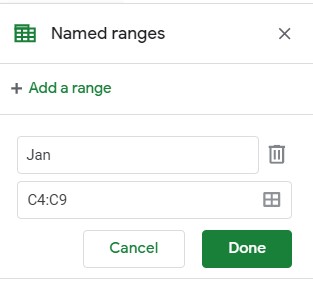
- Click Done.
- Repeat the process for all the months, and all the sales reps
- Once you have created the range names, you can use them in the same way as you used them in Excel.
- Drag the formula across to February and March.
- Repeat for the AVERAGE, MIN and MAX functions.
- We can then amend the names in row 3 to get the totals for 3 of the sales reps. The formulas will automatically pick up the correct values due to the INDIRECT
Excel formulas allow you to identify relationships between values in your spreadsheet’s cells, perform mathematical calculations with those values, and return the resulting value in the cell of your choice. Sum, subtraction, percentage, division, average, and even dates/times are among the formulas that can be performed automatically. For example, =A1+A2+A3+A4+A5, which finds the sum of the range of values from cell A1 to cell A5.
Excel Functions: A formula is a mathematical expression that computes the value of a cell. Functions are predefined formulas that are already in Excel. Functions carry out specific calculations in a specific order based on the values specified as arguments or parameters. For example, =SUM (A1:A10). This function adds up all the values in cells A1 through A10.
How to Insert Formulas in Excel?
This horizontal menu, shown below, in more recent versions of Excel allows you to find and insert Excel formulas into specific cells of your spreadsheet. On the Formulas tab, you can find all available Excel functions in the Function Library:
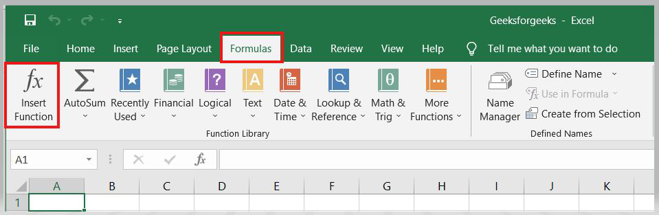
The more you use Excel formulas, the easier it will be to remember and perform them manually. Excel has over 400 functions, and the number is increasing from version to version. The formulas can be inserted into Excel using the following method:
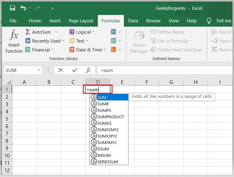
1. Simple insertion of the formula(Typing a formula in the cell):
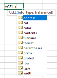
Typing a formula into a cell or the formula bar is the simplest way to insert basic Excel formulas. Typically, the process begins with typing an equal sign followed by the name of an Excel function. Excel is quite intelligent in that it displays a pop-up function hint when you begin typing the name of the function.
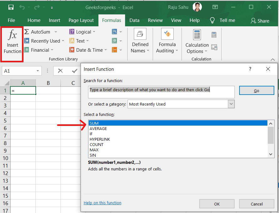
2. Using the Insert Function option on the Formulas Tab:
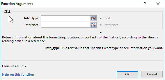
If you want complete control over your function insertion, use the Excel Insert Function dialogue box. To do so, go to the Formulas tab and select the first menu, Insert Function. All the functions will be available in the dialogue box.
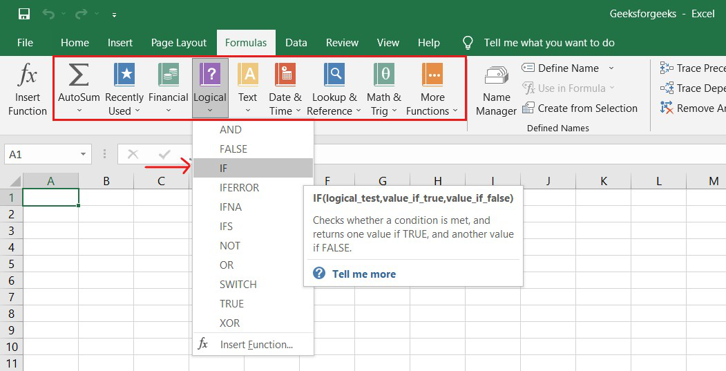
3. Choosing a Formula from One of the Formula Groups in the Formula Tab:
This option is for those who want to quickly dive into their favorite functions. Navigate to the Formulas tab and select your preferred group to access this menu. Click to reveal a sub-menu containing a list of functions. You can then choose your preference. If your preferred group isn’t on the tab, click the More Functions option — it’s most likely hidden there.
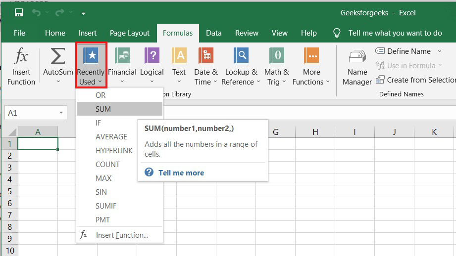
4. Use Recently Used Tabs for Quick Insertion:
If retyping your most recent formula becomes tedious, use the Recently Used menu. It’s on the Formulas tab, the third menu option after AutoSum.
Basic Excel Formulas and Functions:
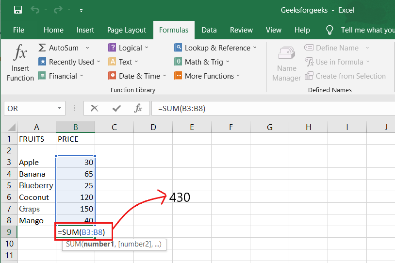
1. SUM:
The SUM formula in Excel is one of the most fundamental formulas you can use in a spreadsheet, allowing you to calculate the sum (or total) of two or more values. To use the SUM formula, enter the values you want to add together in the following format: =SUM(value 1, value 2,…..).
Example: In the below example to calculate the sum of price of all the fruits, in B9 cell type =SUM(B3:B8). this will calculate the sum of B3, B4, B5, B6, B7, B8 Press “Enter,” and the cell will produce the sum: 430.
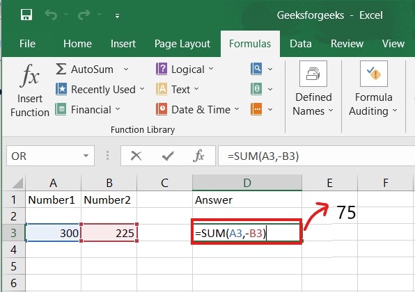
2. SUBTRACTION:
To use the subtraction formula in Excel, enter the cells you want to subtract in the format =SUM (A1, -B1). This will subtract a cell from the SUM formula by appending a negative sign before the cell being subtracted.
For example, if A3 was 300 and B3 was 225, =SUM(A1, -B1) would perform 300 + -225, returning a value of 75 in D3 cell.
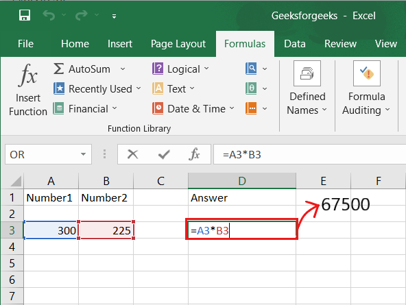
3. MULTIPLICATION:
In Excel, enter the cells to be multiplied in the format =A3*B3 to perform the multiplication formula. An asterisk is used in this formula to multiply cell A3 by cell B3.
For example, if A3 was 300 and B3 was 225, =A1*B1 would return a value of 67500.
Highlight an empty cell in an Excel spreadsheet to multiply two or more values. Then, in the format =A1*B1…, enter the values or cells you want to multiply together. The asterisk effectively multiplies each value in the formula.
To return your desired product, press Enter. Take a look at the screenshot above to see how this looks.
4. DIVISION:
To use the division formula in Excel, enter the dividing cells in the format =A3/B3. This formula divides cell A3 by cell B3 with a forward slash, “/.”
For example, if A3 was 300 and B3 was 225, =A3/B3 would return a decimal value of 1.333333333.
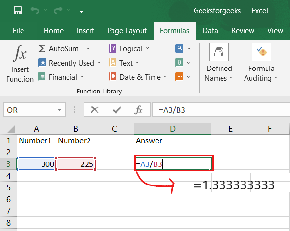
Division in Excel is one of the most basic functions available. To do so, highlight an empty cell, enter an equals sign, “=,” and then the two (or more) values you want to divide, separated by a forward slash, “/.” The output should look like this: =A3/B3, as shown in the screenshot above.
5. AVERAGE:
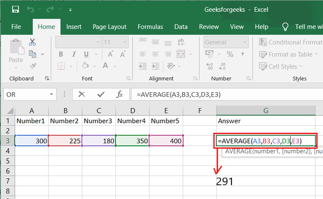
The AVERAGE function finds an average or arithmetic mean of numbers. to find the average of the numbers type = AVERAGE(A3.B3,C3….) and press ‘Enter’ it will produce average of the numbers in the cell.
For example, if A3 was 300, B3 was 225, C3 was 180, D3 was 350, E3 is 400 then =AVERAGE(A3,B3,C3,D3,E3) will produce 291.
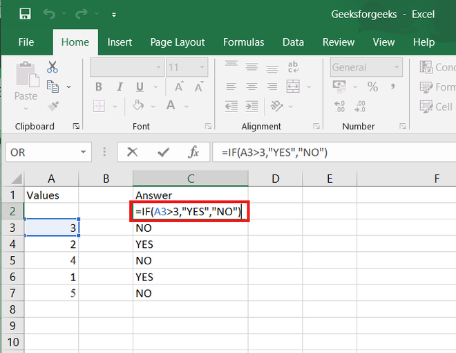
6. IF formula:
In Excel, the IF formula is denoted as =IF(logical test, value if true, value if false). This lets you enter a text value into a cell “if” something else in your spreadsheet is true or false.
For example, You may need to know which values in column A are greater than three. Using the =IF formula, you can quickly have Excel auto-populate a “yes” for each cell with a value greater than 3 and a “no” for each cell with a value less than 3.
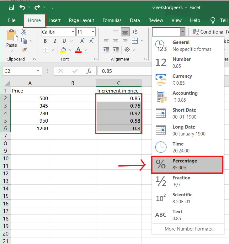
7. PERCENTAGE:
To use the percentage formula in Excel, enter the cells you want to calculate the percentage for in the format =A1/B1. To convert the decimal value to a percentage, select the cell, click the Home tab, and then select “Percentage” from the numbers dropdown.
There isn’t a specific Excel “formula” for percentages, but Excel makes it simple to convert the value of any cell into a percentage so you don’t have to calculate and reenter the numbers yourself.
The basic setting for converting a cell’s value to a percentage is found on the Home tab of Excel. Select this tab, highlight the cell(s) you want to convert to a percentage, and then select Conditional Formatting from the dropdown menu (this menu button might say “General” at first). Then, from the list of options that appears, choose “Percentage.” This will convert the value of each highlighted cell into a percentage. This feature can be found further down.
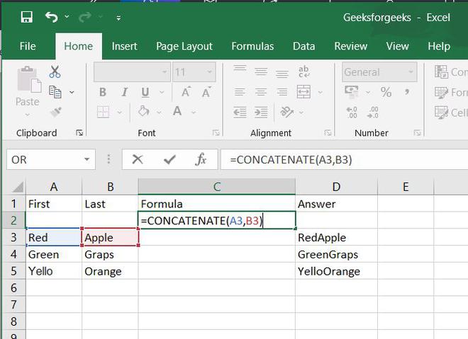
8. CONCATENATE:
CONCATENATE is a useful formula that combines values from multiple cells into the same cell.
For example , =CONCATENATE(A3,B3) will combine Red and Apple to produce RedApple.
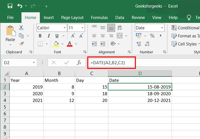
9. DATE:
DATE is the Excel DATE formula =DATE(year, month, day). This formula will return a date corresponding to the values entered in the parentheses, including values referred to from other cells.. For example, if A2 was 2019, B2 was 8, and C1 was 15, =DATE(A1,B1,C1) would return 15-08-2019.
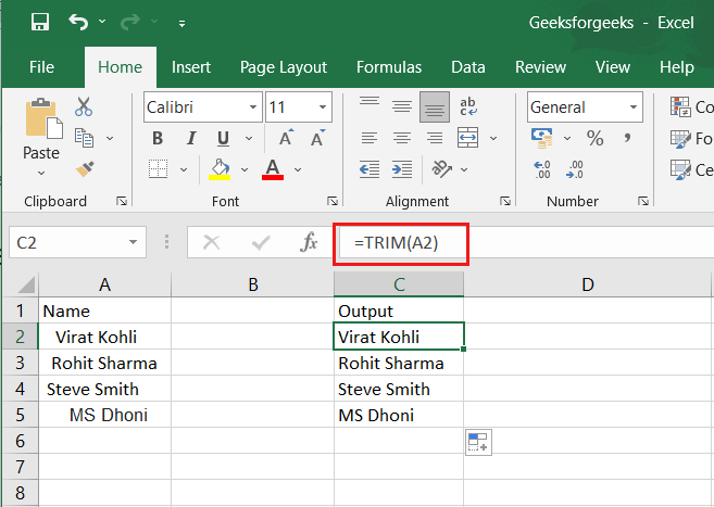
10. TRIM:
The TRIM formula in Excel is denoted =TRIM(text). This formula will remove any spaces that have been entered before and after the text in the cell. For example, if A2 includes the name ” Virat Kohli” with unwanted spaces before the first name, =TRIM(A2) would return “Virat Kohli” with no spaces in a new cell.
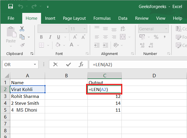
11. LEN:
LEN is the function to count the number of characters in a specific cell when you want to know the number of characters in that cell. =LEN(text) is the formula for this. Please keep in mind that the LEN function in Excel counts all characters, including spaces:
For example,=LEN(A2), returns the total length of the character in cell A2 including spaces.
Excel has a number of formulas that help you use your data in useful ways. For example, you can get an output based on whether or not a cell meets certain specifications. Right now, we’ll focus on a function called “if cell contains, then”. Let’s look at an example.
Jump To Specific Section:
- Explanation: If Cell Contains
- If cell contains any value, then return a value
- If cell contains text/number, then return a value
- If cell contains specific text, then return a value
- If cell contains specific text, then return a value (case-sensitive)
- If cell does not contain specific text, then return a value
- If cell contains one of many text strings, then return a value
- If cell contains several of many text strings, then return a value
Excel Formula: If cell contains
Generic formula
=IF(ISNUMBER(SEARCH("abc",A1)),A1,"")
Summary
To test for cells that contain certain text, you can use a formula that uses the IF function together with the SEARCH and ISNUMBER functions. In the example shown, the formula in C5 is:
=IF(ISNUMBER(SEARCH("abc",B5)),B5,"")
If you want to check whether or not the A1 cell contains the text “Example”, you can run a formula that will output “Yes” or “No” in the B1 cell. There are a number of different ways you can put these formulas to use. At the time of writing, Excel is able to return the following variations:
- If cell contains any value
- If cell contains text
- If cell contains number
- If cell contains specific text
- If cell contains certain text string
- If cell contains one of many text strings
- If cell contains several strings
Using these scenarios, you’re able to check if a cell contains text, value, and more.
Explanation: If Cell Contains
One limitation of the IF function is that it does not support Excel wildcards like «?» and «*». This simply means you can’t use IF by itself to test for text that may appear anywhere in a cell.
One solution is a formula that uses the IF function together with the SEARCH and ISNUMBER functions. For example, if you have a list of email addresses, and want to extract those that contain «ABC», the formula to use is this:
=IF(ISNUMBER(SEARCH("abc",B5)),B5,""). Assuming cells run to B5
If «abc» is found anywhere in a cell B5, IF will return that value. If not, IF will return an empty string («»). This formula’s logical test is this bit:
ISNUMBER(SEARCH("abc",B5))
Read article: Excel efficiency: 11 Excel Formulas To Increase Your Productivity
Using “if cell contains” formulas in Excel
The guides below were written using the latest Microsoft Excel 2019 for Windows 10. Some steps may vary if you’re using a different version or platform. Contact our experts if you need any further assistance.
1. If cell contains any value, then return a value
This scenario allows you to return values based on whether or not a cell contains any value at all. For example, we’ll be checking whether or not the A1 cell is blank or not, and then return a value depending on the result.
- Select the output cell, and use the following formula: =IF(cell<>»», value_to_return, «»).
- For our example, the cell we want to check is A2, and the return value will be No. In this scenario, you’d change the formula to =IF(A2<>»», «No», «»).
- Since the A2 cell isn’t blank, the formula will return “No” in the output cell. If the cell you’re checking is blank, the output cell will also remain blank.
2. If cell contains text/number, then return a value
With the formula below, you can return a specific value if the target cell contains any text or number. The formula will ignore the opposite data types.
Check for text
- To check if a cell contains text, select the output cell, and use the following formula: =IF(ISTEXT(cell), value_to_return, «»).
- For our example, the cell we want to check is A2, and the return value will be Yes. In this scenario, you’d change the formula to =IF(ISTEXT(A2), «Yes», «»).

- Because the A2 cell does contain text and not a number or date, the formula will return “Yes” into the output cell.
Check for a number or date
- To check if a cell contains a number or date, select the output cell, and use the following formula: =IF(ISNUMBER(cell), value_to_return, «»).
- For our example, the cell we want to check is D2, and the return value will be Yes. In this scenario, you’d change the formula to =IF(ISNUMBER(D2), «Yes», «»).

- Because the D2 cell does contain a number and not text, the formula will return “Yes” into the output cell.
3. If cell contains specific text, then return a value
To find a cell that contains specific text, use the formula below.
- Select the output cell, and use the following formula: =IF(cell=»text», value_to_return, «»).
- For our example, the cell we want to check is A2, the text we’re looking for is “example”, and the return value will be Yes. In this scenario, you’d change the formula to =IF(A2=»example», «Yes», «»).

- Because the A2 cell does consist of the text “example”, the formula will return “Yes” into the output cell.
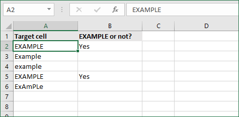
4. If cell contains specific text, then return a value (case-sensitive)
To find a cell that contains specific text, use the formula below. This version is case-sensitive, meaning that only cells with an exact match will return the specified value.
- Select the output cell, and use the following formula: =IF(EXACT(cell,»case_sensitive_text»), «value_to_return», «»).
- For our example, the cell we want to check is A2, the text we’re looking for is “EXAMPLE”, and the return value will be Yes. In this scenario, you’d change the formula to =IF(EXACT(A2,»EXAMPLE»), «Yes», «»).
- Because the A2 cell does consist of the text “EXAMPLE” with the matching case, the formula will return “Yes” into the output cell.
5. If cell does not contain specific text, then return a value
The opposite version of the previous section. If you want to find cells that don’t contain a specific text, use this formula.
- Select the output cell, and use the following formula: =IF(cell=»text», «», «value_to_return»).
- For our example, the cell we want to check is A2, the text we’re looking for is “example”, and the return value will be No. In this scenario, you’d change the formula to =IF(A2=»example», «», «No»).
- Because the A2 cell does consist of the text “example”, the formula will return a blank cell. On the other hand, other cells return “No” into the output cell.
6. If cell contains one of many text strings, then return a value
This formula should be used if you’re looking to identify cells that contain at least one of many words you’re searching for.
- Select the output cell, and use the following formula: =IF(OR(ISNUMBER(SEARCH(«string1», cell)), ISNUMBER(SEARCH(«string2», cell))), value_to_return, «»).
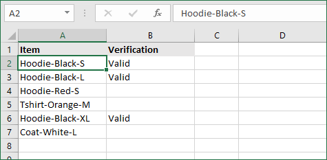
- For our example, the cell we want to check is A2. We’re looking for either “tshirt” or “hoodie”, and the return value will be Valid. In this scenario, you’d change the formula to =IF(OR(ISNUMBER(SEARCH(«tshirt»,A2)),ISNUMBER(SEARCH(«hoodie»,A2))),»Valid «,»»).
- Because the A2 cell does contain one of the text values we searched for, the formula will return “Valid” into the output cell.
To extend the formula to more search terms, simply modify it by adding more strings using ISNUMBER(SEARCH(«string», cell)).
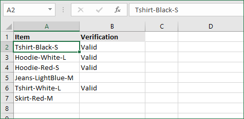
7. If cell contains several of many text strings, then return a value
This formula should be used if you’re looking to identify cells that contain several of the many words you’re searching for. For example, if you’re searching for two terms, the cell needs to contain both of them in order to be validated.
- Select the output cell, and use the following formula: =IF(AND(ISNUMBER(SEARCH(«string1»,cell)), ISNUMBER(SEARCH(«string2″,cell))), value_to_return,»»).
- For our example, the cell we want to check is A2. We’re looking for “hoodie” and “black”, and the return value will be Valid. In this scenario, you’d change the formula to =IF(AND(ISNUMBER(SEARCH(«hoodie»,A2)),ISNUMBER(SEARCH(«black»,A2))),»Valid «,»»).
- Because the A2 cell does contain both of the text values we searched for, the formula will return “Valid” to the output cell.
Final thoughts
We hope this article was useful to you in learning how to use “if cell contains” formulas in Microsoft Excel. Now, you can check if any cells contain values, text, numbers, and more. This allows you to navigate, manipulate and analyze your data efficiently.
We’re glad you’re read the article up to here  Thank you
You may also like
» How to use NPER Function in Excel
» How to Separate First and Last Name in Excel
» How to Calculate Break-Even Analysis in Excel
Very often, when working in Excel, you need to use data about addressing cells in a spreadsheet. For this was provided the function CELL. Consider its use on specific examples.
Function CELL value and properties in Excel
It should be noted that Excel uses several functions for addressing cells:
- — ROW;
- — COLUMN and others.
CELL function return information about the formatting, address, or contents of a cell. The function can return detailed information about the cell format, thereby eliminating the need to use VBA in some cases. The function is especially useful if you need to display the full path of the file in the cells.
How does the CELL function in Excel work?
Function in its work uses the syntax that consists of two arguments:
=CELL(info_type,[reference])
- Info_type is a text value that specifies the type of cell information that is required. When you enter a function manually, a drop-down list is displayed where all possible values of the “information type” argument are shown:
- [Reference] is an optional argument. The cell for which you want to receive information. If this argument is omitted, the information specified in the information_type argument is returned for the last cell changed. If the link argument points to a range of cells, function returns information only for the upper-left value of the range.
Examples of using the CELL function in Excel
Example 1. Given the table of accounting work of employees of the organization of the form:
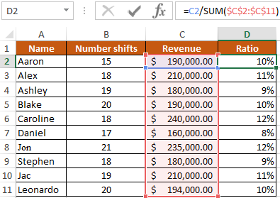
It is necessary with the help of the CELL function to calculate in which row and column the salary is in the amount of 235,000 dollars.
To do this, we introduce the following formula:
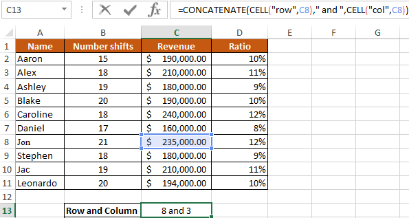
here:
- — «row» and «column» — output parameter;
- — C8 — address data with a salary.
As a result of the calculations, we obtain: row №8 and column № 3 (C).
How to know width of an Excel spreadsheet?
Example 2. It is necessary to calculate the width of the table in characters. Immediately it should be noted that in Excel, by default, the width of columns and cells is measured in the number of characters that they fit in their value are available for display in a cell without a line break.
Note. The height of lines and cells in Excel is by default measured in units of the basic font — in (pt) points. The larger the font, the higher the line for full display of characters in height.
Let’s enter into C14 the formula for calculating the sum of the width of each column of the table:
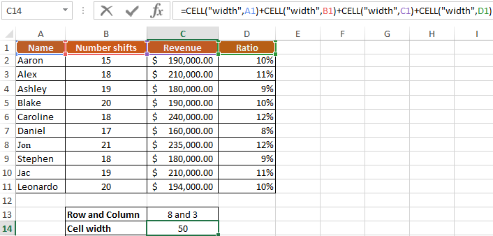
here:
- — «width» is a function parameter;
- — A1 — the width of a specific column.
How to get the value of the first value in the range
Example 3. In the condition of example 1, you need to display the contents of only the first (upper left) value from the range A5:C8.
We introduce the formula for calculating:
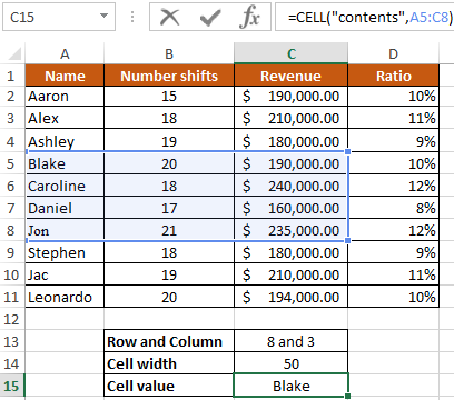
Download examples CELL function in Excel
Description of the formula is similar to the previous two examples.