
Excel for Microsoft 365 Excel for Microsoft 365 for Mac Excel for the web Excel 2021 Excel 2021 for Mac Excel 2019 Excel 2019 for Mac Excel 2016 Excel 2016 for Mac Excel 2013 Excel for iPad Excel for iPhone Excel for Android tablets Excel 2010 Excel 2007 Excel for Mac 2011 Excel for Android phones Excel Starter 2010 More…Less
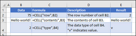
The CELL function returns information about the formatting, location, or contents of a cell. For example, if you want to verify that a cell contains a numeric value instead of text before you perform a calculation on it, you can use the following formula:
=IF(CELL(«type»,A1)=»v»,A1*2,0)
This formula calculates A1*2 only if cell A1 contains a numeric value, and returns 0 if A1 contains text or is blank.
Note: Formulas that use CELL have language-specific argument values and will return errors if calculated using a different language version of Excel. For example, if you create a formula containing CELL while using the Czech version of Excel, that formula will return an error if the workbook is opened using the French version. If it is important for others to open your workbook using different language versions of Excel, consider either using alternative functions or allowing others to save local copies in which they revise the CELL arguments to match their language.
Syntax
CELL(info_type, [reference])
The CELL function syntax has the following arguments:
|
Argument |
Description |
|---|---|
|
info_type Required |
A text value that specifies what type of cell information you want to return. The following list shows the possible values of the Info_type argument and the corresponding results. |
|
reference Optional |
The cell that you want information about. If omitted, the information specified in the info_type argument is returned for cell selected at the time of calculation. If the reference argument is a range of cells, the CELL function returns the information for active cell in the selected range. Important: Although technically reference is optional, including it in your formula is encouraged, unless you understand the effect its absence has on your formula result and want that effect in place. Omitting the reference argument does not reliably produce information about a specific cell, for the following reasons:
|
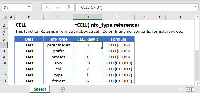
info_type values
The following list describes the text values that can be used for the info_type argument. These values must be entered in the CELL function with quotes (» «).
|
info_type |
Returns |
|---|---|
|
«address» |
Reference of the first cell in reference, as text. |
|
«col» |
Column number of the cell in reference. |
|
«color» |
The value 1 if the cell is formatted in color for negative values; otherwise returns 0 (zero). Note: This value is not supported in Excel for the web, Excel Mobile, and Excel Starter. |
|
«contents» |
Value of the upper-left cell in reference; not a formula. |
|
«filename» |
Filename (including full path) of the file that contains reference, as text. Returns empty text («») if the worksheet that contains reference has not yet been saved. Note: This value is not supported in Excel for the web, Excel Mobile, and Excel Starter. |
|
«format» |
Text value corresponding to the number format of the cell. The text values for the various formats are shown in the following table. Returns «-» at the end of the text value if the cell is formatted in color for negative values. Returns «()» at the end of the text value if the cell is formatted with parentheses for positive or all values. Note: This value is not supported in Excel for the web, Excel Mobile, and Excel Starter. |
|
«parentheses» |
The value 1 if the cell is formatted with parentheses for positive or all values; otherwise returns 0. Note: This value is not supported in Excel for the web, Excel Mobile, and Excel Starter. |
|
«prefix» |
Text value corresponding to the «label prefix» of the cell. Returns single quotation mark (‘) if the cell contains left-aligned text, double quotation mark («) if the cell contains right-aligned text, caret (^) if the cell contains centered text, backslash () if the cell contains fill-aligned text, and empty text («») if the cell contains anything else. Note: This value is not supported in Excel for the web, Excel Mobile, and Excel Starter. |
|
«protect» |
The value 0 if the cell is not locked; otherwise returns 1 if the cell is locked. Note: This value is not supported in Excel for the web, Excel Mobile, and Excel Starter. |
|
«row» |
Row number of the cell in reference. |
|
«type» |
Text value corresponding to the type of data in the cell. Returns «b» for blank if the cell is empty, «l» for label if the cell contains a text constant, and «v» for value if the cell contains anything else. |
|
«width» |
Returns an array with 2 items. The 1st item in the array is the column width of the cell, rounded off to an integer. Each unit of column width is equal to the width of one character in the default font size. The 2nd item in the array is a Boolean value, the value is TRUE if the column width is the default or FALSE if the width has been explicitly set by the user. Note: This value is not supported in Excel for the web, Excel Mobile, and Excel Starter. |
CELL format codes
The following list describes the text values that the CELL function returns when the Info_type argument is «format» and the reference argument is a cell that is formatted with a built-in number format.
|
If the Excel format is |
The CELL function returns |
|---|---|
|
General |
«G» |
|
0 |
«F0» |
|
#,##0 |
«,0» |
|
0.00 |
«F2» |
|
#,##0.00 |
«,2» |
|
$#,##0_);($#,##0) |
«C0» |
|
$#,##0_);[Red]($#,##0) |
«C0-« |
|
$#,##0.00_);($#,##0.00) |
«C2» |
|
$#,##0.00_);[Red]($#,##0.00) |
«C2-« |
|
0% |
«P0» |
|
0.00% |
«P2» |
|
0.00E+00 |
«S2» |
|
# ?/? or # ??/?? |
«G» |
|
m/d/yy or m/d/yy h:mm or mm/dd/yy |
«D4» |
|
d-mmm-yy or dd-mmm-yy |
«D1» |
|
d-mmm or dd-mmm |
«D2» |
|
mmm-yy |
«D3» |
|
mm/dd |
«D5» |
|
h:mm AM/PM |
«D7» |
|
h:mm:ss AM/PM |
«D6» |
|
h:mm |
«D9» |
|
h:mm:ss |
«D8» |
Note: If the info_type argument in the CELL function is «format» and you later apply a different format to the referenced cell, you must recalculate the worksheet (press F9) to update the results of the CELL function.
Examples
Need more help?
You can always ask an expert in the Excel Tech Community or get support in the Answers community.
See Also
Change the format of a cell
Create or change a cell reference
ADDRESS function
Add, change, find or clear conditional formatting in a cell
Need more help?
In this example, the goal is to test the passwords in column B to see if they contain a number. This is a surprisingly tricky problem because Excel doesn’t have a function that will let you test for a number inside a text string directly. Note this is different from checking if a cell value is a number. You can easily perform that test with the ISNUMBER function. In this case, however, we to test if a cell value contains a number, which may occur anywhere. One solution is to use the FIND function with an array constant. In Excel 365, which supports dynamic array formulas, you can use a different formula based on the SEQUENCE function. Both approaches are explained below.
FIND function
The FIND function is designed to look inside a text string for a specific substring. If FIND finds the substring, it returns a position of the substring in the text as a number. If the substring is not found, FIND returns a #VALUE error. For example:
=FIND("p","apple") // returns 2
=FIND("z","apple") // returns #VALUE!
We can use this same idea to check for numbers as well:
=FIND(3,"app637") // returns 5
=FIND(9,"app637") // returns #VALUE!
The challenge in this case is that we need to check the values in column B for ten different numbers, 0-9. One way to do that is to supply these numbers as the array constant {0,1,2,3,4,5,6,7,8,9}. This is the approach taken in the formula in cell D5:
=COUNT(FIND({0,1,2,3,4,5,6,7,8,9},B5))>0Inside the COUNT function, the FIND function is configured to look for all ten numbers in cell B5:
FIND({0,1,2,3,4,5,6,7,8,9},B5)Because we are giving FIND ten values to look for, it returns an array with 10 results. In other words, FIND checks the text in B5 for each number and returns all results at once:
{#VALUE!,4,5,6,#VALUE!,#VALUE!,#VALUE!,#VALUE!,#VALUE!,#VALUE!}Unless you look at arrays often, this may look pretty cryptic. Here is the translation: The number 1 was found at position 4, the number 2 was found at position 5, and the number 3 was found at position 6. All other numbers were not found and returned #VALUE errors.
We are very close now to a final formula. We simply need to tally up results. To do this, we nest the FIND formula above inside the COUNT function like this:
=COUNT(FIND({0,1,2,3,4,5,6,7,8,9},B5))FIND returns the array of results directly to COUNT, which counts the numbers in the array. COUNT only counts numeric values, and ignores errors. This means COUNT will return a number greater than zero if there are any numbers in the value being tested. In the case of cell B5, COUNT returns 3.
The last step is to check the result from COUNT and force a TRUE or FALSE result. We do this by adding «>0» to the end of formula:
=COUNT(FIND({0,1,2,3,4,5,6,7,8,9},B5))>0Now the formula will return TRUE or FALSE. To display a custom result, you can use the IF function:
=IF(COUNT(FIND({0,1,2,3,4,5,6,7,8,9},B5))>0, "Yes", "No")
The original formula is now nested inside IF as the logical_test argument. This formula will return «Yes» if B5 contains a number and «No» if not.
SEQUENCE function
In Excel 365, which offers dynamic array formulas, we can take a different approach to this problem.
=COUNT(--MID(B5,SEQUENCE(LEN(B5)),1))>0This isn’t necessarily a better approach, just a different way to solve the same problem. At the core, this formula uses the MID function together with the SEQUENCE function to split the text in cell B5 into an array:
MID(B5,SEQUENCE(LEN(B5)),1)Working from the inside out, the LEN function returns the length of the text in cell B5:
LEN(B5) // returns 6This number is returned to the SEQUENCE function as the rows argument, and SEQUENCE returns an array of numbers, 1-6:
=SEQUENCE(LEN(B5))
=SEQUENCE(6)
={1;2;3;4;5;6}
This array is returned to the MID function as the start_num argument, and, with num_chars set to 1, the MID function returns an array that contains the characters in cell B5:
=MID(B5,{1;2;3;4;5;6},1)
={"a";"b";"c";"1";"2";"3"}
We can now simplify the original formula to:
=COUNT(--{"a";"b";"c";"1";"2";"3"})>0We use the double-negative (—) to get Excel to try and coerce the values in the array into numbers. The result looks like this:
=COUNT({#VALUE!;#VALUE!;#VALUE!;1;2;3})>0The math operation created by the double negative (—) returns an actual number when successful and a #VALUE! error when the operation fails. The COUNT function counts the numbers, ignoring any errors, and returns 3. As above, we check the final count with «>0», and the result for cell B5 is TRUE.
Note: as you might guess, you can easily adapt this formula to count numbers in a text string.
Cell equals number?
Note that the formulas above are too complex if you only want to test if a cell equals a number. In that case, you can simply use the ISNUMBER function like this:
=ISNUMBER(A1)
This Tutorial demonstrates how to use the Excel CELL Function in Excel to get information about a cell.
CELL Function Overview
The CELL Function Returns information about a cell. Color, filename, contents, format, row, etc.
To use the CELL Excel Worksheet Function, select a cell and type:
![]()
(Notice how the formula inputs appear)
CELL function Syntax and inputs:
=CELL(info_type,reference)info_type – Text indicating what cell information you would like to return.
reference – The cell reference that you want information about.
How to use the CELL Function in Excel
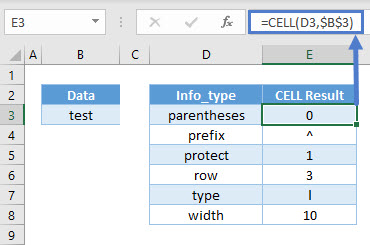
The CELL Function returns information about the formatting, location, or contents of cell.
=CELL(D3,$B$3)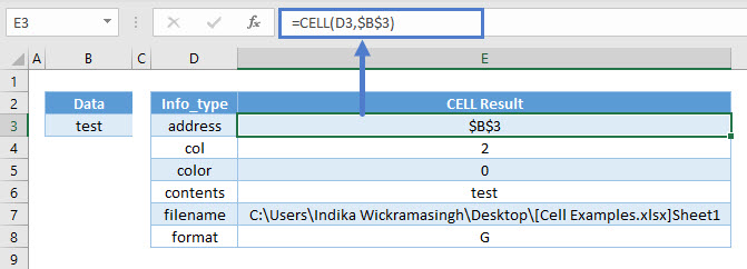
As seen above, the CELL Function returns all kinds of information from cell B3.
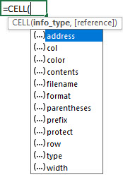
If you type =CELL(, you will be able to see 12 different types of information to retrieve.
Here are additional outputs of the CELL Function:
Overall View of Info_types
Some of the info_types are pretty straightforward and retrieves what you asked for, while the rest will be explained in the next few sections because of the complexity.
| Info_type | What it retrieves? |
| “address” | The cell reference/address. |
| “col” | The column number. |
| “color” | * |
| “contents” | The value itself or result of the formula. |
| “filename” | The full path, filename, and extension in square brackets, and sheet name. |
| “format” | * |
| “parentheses” | * |
| “prefix” | * |
| “protect” | * |
| “row” | The row number. |
| “type” | * |
| “width” | The column width rounded to the nearest integer. |
* Explained in the next few sections.
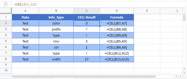
Color Info_type
Color will show all results as 0 unless the cell is formatted with color for negative values. The latter will show as 1.
=CELL("color",B3)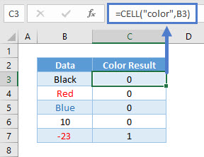
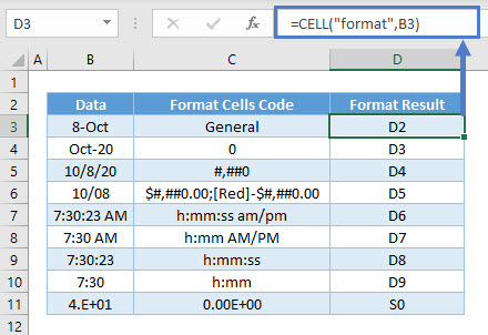
Format Info_type
Format shows the number format of the cell, but it might not be what you expect.
=CELL("format",B3)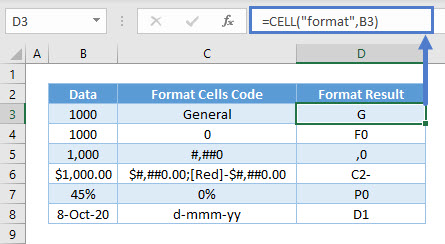
There are many kinds of different variations with formatting, but here are some guidelines to figure it out:
- “G” is for General, “C” for Currency, “P” for Percentage, “S” for Scientific (not shown above), “D” for Date.
- If the digits are with numbers, currencies, and percentages; it represents the decimal places. Eg. “F0” means 0 decimals in cell D4, and “C2-” means 2 decimals in cell D6. “D1” in cell D8 is simply a type of date format (there are D1 to D9 for different kinds of date and time formats).
- A comma at the beginning is for thousand separators (“,0” in cell D5 for eg).
- A minus sign is for formatting negative values with a color (“C2-” in cell D6 for eg).
Here are other examples of date formats and for scientific.
Parentheses Info_type
Parentheses shows 1 if the cell is formatted with parentheses (either or both positive and negative). Otherwise, it shows 0.
=CELL("parentheses",B3)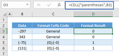
Prefix Info_type
Prefix results in various symbols depending on how the text is aligned in the cell.
=CELL("prefix",B3)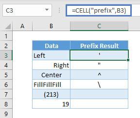
As seen above, a left alignment of the text is a single quote in cell C3.
A right alignment of the text shows double quotes in cell C4.
A center alignment of the text shows caret in cell C5.
A fill alignment of the text shows backslash in cell C6.
Numbers (cell C7 and C8) show as blank regardless of alignment.
Protect Info_type
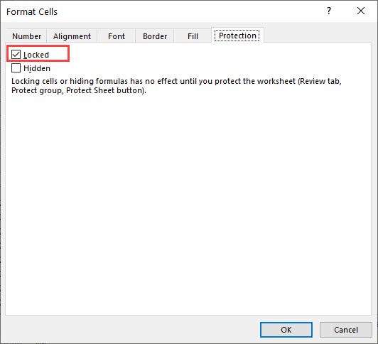
Protect results in 1 if the cell is locked, and 0 if it’s unlocked.
=CELL("protect",B3)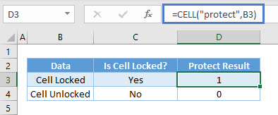
Do note that all cells are locked by default. That is why you can’t edit any cells after you protect it. To unlock it, right-click on a cell and choose Format Cells.
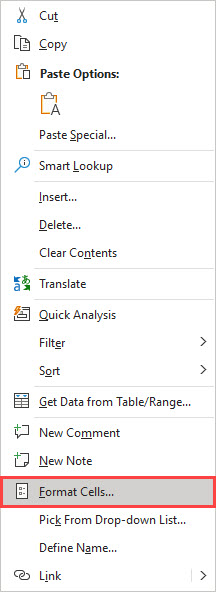
Go to the Protection tab and you can uncheck “Locked” to unlock the cell.
Type Info_type
Type results in three different alphabets dependent on the data type in the cell.
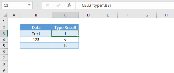
“l” stands for label in cell C3.
“v” stands for value in cell C4.
“b” stands for blank in cell C5.
Create Hyperlink to Lookup Using Address
You can use the CELL Function along with HYPERLINK and INDEX / MATCH to hyperlink to a lookup result:
=HYPERLINK("#"&CELL("address",INDEX(C3:C6,MATCH("mango",B3:B6,0))),INDEX(C3:C6,MATCH("mango",B3:B6,0)))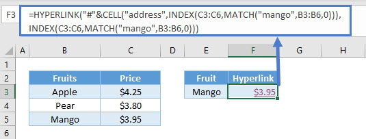
The INDEX and MATCH formula retrieves the price of Mango in cell C5: $3.95. The CELL Function, with “address” returns the cell location. The HYPERLINK function then creates the hyperlink.
Retrieve File Path
To retrieve the file path where the particular file is stored, you can use:
=LEFT(CELL("filename"),FIND("[",CELL("filename"))-1)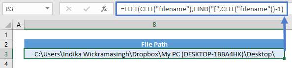
Since the filename will be the same using any cell reference, you can omit it. Use FIND function to obtain the position where “[“ starts and minus 1 to allow LEFT function to retrieve the characters before that.
Retrieve File Name
To retrieve the file name, you can use:
=MID(CELL("filename"),FIND("[",CELL("filename"))+1,FIND("]",CELL("filename"))-FIND("[",CELL("filename"))-1)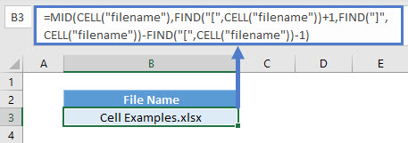
This uses a similar concept as above where FIND function obtains the position where “[“ starts and retrieves the characters after that. To know how many characters to extract, it uses the position of “]” minus “[“ and minus 1 as it includes the position of “]”.
Retrieve Sheet Name
To retrieve the sheet name, you can use:
=MID(CELL("filename"),FIND("]",CELL("filename"))+1,LEN(CELL("filename")))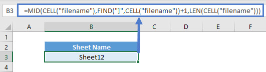
Again, it’s similar to the above where FIND function obtains the position where “]“ starts and retrieves the characters after that. To know how many characters to extract, it uses the total length of what “filename” info_type returns.
CELL Function in Google Sheets
The CELL function works similarly in Google Sheets. It just doesn’t have the full range of info_type. It only includes “address”, “col”, “color”, “contents”, “prefix”, “row”, “type”, and “width”.
Additional Notes
The CELL Function returns information about a cell. The information that can be returned relates to cell location, formatting and contents.
Enter the type of information you want then enter the cell reference for the cell you want information about.
Return to the List of all Functions in Excel
How to get the row or column number of the current cell or any other cell in Excel.
This tutorial covers important functions that allow you to do everything from alternate row and column shading to incrementing values at specified intervals and much more.
We will use the ROW and COLUMN function for this. Here is an example of the output from these functions.
Though this doesn’t look like much, these functions allow for the creation of powerful formulas when combined with other functions. Now, let’s look at how to create them.
Get a Cell’s Row Number
Syntax
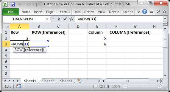
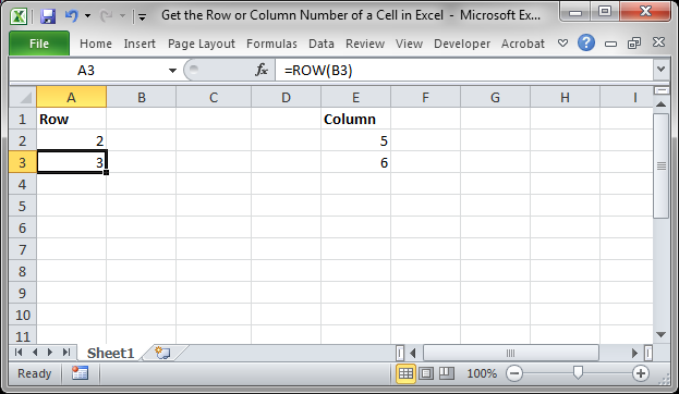
This function returns the number of the row that a particular cell is in.
If you leave the function empty, it will return the row number for the current cell in which this function has been placed.
If you put a cell reference within this function, it will return the row number for that cell reference.
This example would return 1 since cell A1 is in row 1. If it was =ROW(C24) the function would return the number 24 because cell C24 is in row 24.
Examples
Now that you know how this function works, it may seem rather useless. Here are links to two examples where this function is key.
Increment a Value Every X Number of Rows in Excel
Shade Every Other Row in Excel Quickly
Get a Cell’s Column Number
Syntax
This function returns the number of the column that a particular cell is in. It counts from left to right, where A is 1 and B is 2 and so on.
If you leave the function empty, it will return the column number for the current cell in which this function has been placed.
If you put a cell reference within this function, it will return the column number for that cell reference.
This example would return 1 since cell A1 is in row 1. If it was =COLUMN (C24) the function would return the number 3 because cell C24 is in column number 3.
Examples
The COLUMN function works just like the ROW function does except that it works on columns, going left to right, whereas the ROW function works on rows, going up and down.
As such, almost every example where ROW is used could be converted to use COLUMN based on your needs.
Notes
The ROW and COLUMN functions are building blocks in that they help you create more complex formulas in Excel. Alone, these functions are pretty much worthless, but, if you can memorize them and keep them for later, you will start to find more and more uses for them when working in large data sets. The examples provided above in the ROW section cover only two of many different ways you can use these functions to create more powerful and helpful spreadsheets.
Similar Content on TeachExcel
Sum Values from Every X Number of Rows in Excel
Tutorial: Add values from every x number of rows in Excel. For instance, add together every other va…
Formulas to Remove First or Last Character from a Cell in Excel
Tutorial: Formulas that allow you to quickly and easily remove the first or last character from a ce…
Formula to Delete the First or Last Word from a Cell in Excel
Tutorial:
Excel formula to delete the first or last word from a cell.
You can copy and paste the fo…
Reverse the Contents of a Cell in Excel — UDF
Macro: Reverse cell contents with this free Excel UDF (user defined function). This will mir…
Excel Function to Remove All Text OR All Numbers from a Cell
Tutorial: How to create and use a function that removes all text or all numbers from a cell, whichev…
Get the First Word from a Cell in Excel
Tutorial: How to use a formula to get the first word from a cell in Excel. This works for a single c…
Subscribe for Weekly Tutorials
BONUS: subscribe now to download our Top Tutorials Ebook!
Numbering in Excel means providing a cell with numbers like serial numbers to some table. We can also do it manually by filling the first two cells with numbers and dragging them down to the end of the table, which Excel will automatically load the series. Else, we can use the =ROW() formula to insert a row number as the serial number in the data or table.
When working with Excel, some small tasks need to be done repeatedly. However, if we know the right way to do it, they can save a lot of time. For example, generating the numbers in Excel is a task that is often used while working. Serial numbers play a very important role in Excel. It defines a unique identity for each record of your data.
One of the ways is to add the serial numbers manually in Excel. But it can be a pain if you have the data of hundreds or thousands of rows and must enter the row number for them.
This article will cover the different ways to do it.
Table of contents
- Numbering in Excel
- How to Add Serial Number in Excel Automatically?
- #1 – Using Fill Handle
- #2 – Using Fill Series
- #3 – Using the ROW Function
- Things to Remember about Numbering in Excel
- Recommended Articles
How to Add Serial Number in Excel Automatically?
There are many ways to generate the number of rows in Excel.
You can download this Numbering in Excel Template here – Numbering in Excel Template
- Using Fill Handle
- Using Fill Series
- Using ROW Function
#1 – Using Fill Handle
It identifies a pattern from a few already filled cells and then quickly uses that pattern to fill the entire column.
For example, let us take the below dataset.
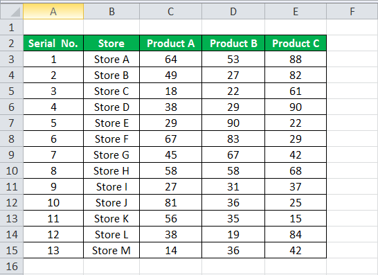
For the above dataset, we have to fill the serial no record-wise. Follow the below steps:
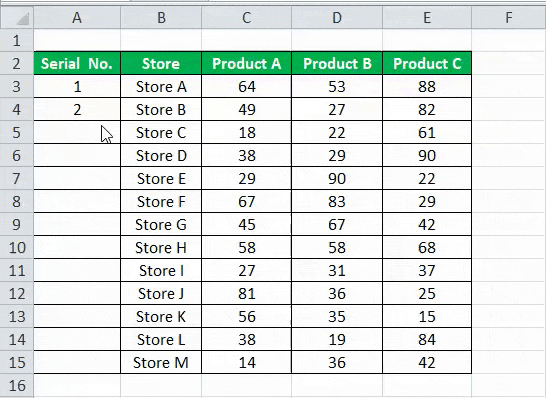
- First, we must enter 1 in cell A3 and insert 2 in cell A4.
- Then, select both the cells as per the below screenshot.

As we can see, a small square is shown in the above screenshot, which is rounded by a red color called “Fill Handle” in Excel.
Place the mouse cursor on this square and double-click on the fill handle.
- It will automatically fill all the cells until the end of the dataset. For example, refer to the below screenshot.

As the fill handle identifies the pattern, fill the individual cells with that pattern.
If you have any blank row in the dataset, the fill handle would only work until the last contiguous non-blank row.

#2 – Using Fill Series
It gives more control over data on how the serial numbers are entered into Excel.
For example, suppose you have below the score of students subject-wise.

Follow the below steps to fill series in the Excel:
- We must first insert 1 in cell A3.
- Then, go to the “HOME” tab. Next, click on the “Fill” option under the “Editing” section, as shown in the below screenshot.

- Click on the “Fill” dropdown. It has many options. Click on “Series,” as shown in the below screenshot.

- It will open a dialog box, as shown below screenshot.

- Click on “Columns” under the “Series in” section. Then, refer to the below screenshot.

- Insert the value under the “Stop value” field. In this case, we have 10 records; enter 10. If we skip this value, the Fill “Series” option may not work.
- Enter “OK.” It will fill rows with serial numbers from 1 to 10. Refer to the below screenshot.

#3 – Using the ROW Function
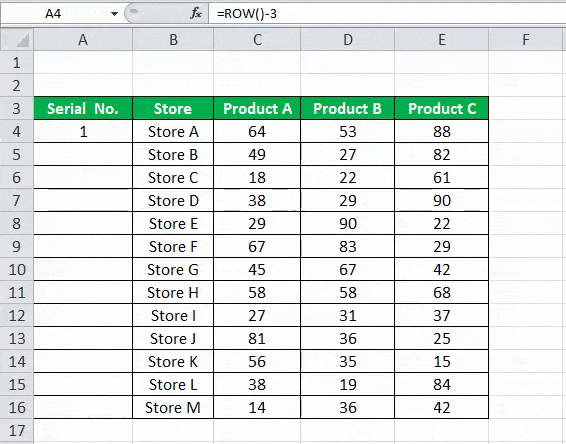
Excel has a built-in function, which also can be used to number the rows in Excel. To get the Excel row numbering, we must enter the following formula in the first cell shown below:

- The ROW function gives the Excel row number of the current row. We have subtracted 3 from it as we started the data from the 4th. If the data starts from the 2nd row, we must remove 1 from it.
- See the below screenshot. Using =ROW()-3 formula.

Drag this formula for the rest of the rows. The final result is shown below.
Using this formula for numbering will not damage the numbers if we delete a record in the dataset. Furthermore, since the ROW function does not reference cell addresses, it will automatically adjust to give the correct row number.
Things to Remember about Numbering in Excel
- The “Fill Handle” and “Fill Series” options are static. Therefore, if we move or delete any record or row in the dataset, the row number will not change accordingly.
- The ROW function gives the exact numbering if we cut and copy the data in Excel.
Recommended Articles
This article is a guide to Numbering in Excel. We discuss how to automatically add serial numbers in Excel using the fill handle, fill series, and ROW function, along with examples and downloadable templates. You may learn more about Excel functions from the following articles: –
- Auto Numbering in ExcelThere are two approaches for auto numbering. To begin, fill the first two cells with the series you wish to insert and drag it to the table’s end. Second, use the =ROW() formula to get the number, and then drag it to the table’s end.read more
- Row Limit in Excel
- Excel Negative NumberIn Excel, negative numbers, i.e. numbers less than 0 in value, are displayed with minus symbols by default.read more
- IsNumber FunctionISNUMBER function in excel is an information function that checks if the referred cell value is numeric or non-numeric.read more
- Null in ExcelNull is a type of error in Excel that occurs when two or more cell references provided in formulas are wrong, or when their position is incorrect. Using space in formulas between two cell references, for example, will result in a null error.read more
Reader Interactions