
Excel for Microsoft 365 Excel for Microsoft 365 for Mac Excel 2021 Excel 2021 for Mac Excel 2019 Excel 2019 for Mac Excel 2016 Excel 2016 for Mac Excel 2013 Excel 2010 Excel 2007 Excel for Mac 2011 More…Less
Sometimes you need to check if a cell is blank, generally because you might not want a formula to display a result without input.

In this case we’re using IF with the ISBLANK function:
-
=IF(ISBLANK(D2),»Blank»,»Not Blank»)
Which says IF(D2 is blank, then return «Blank», otherwise return «Not Blank»). You could just as easily use your own formula for the «Not Blank» condition as well. In the next example we’re using «» instead of ISBLANK. The «» essentially means «nothing».
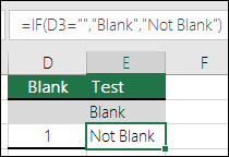
=IF(D3=»»,»Blank»,»Not Blank»)
This formula says IF(D3 is nothing, then return «Blank», otherwise «Not Blank»). Here is an example of a very common method of using «» to prevent a formula from calculating if a dependent cell is blank:
-
=IF(D3=»»,»»,YourFormula())
IF(D3 is nothing, then return nothing, otherwise calculate your formula).
Need more help?
Want more options?
Explore subscription benefits, browse training courses, learn how to secure your device, and more.
Communities help you ask and answer questions, give feedback, and hear from experts with rich knowledge.
The logical expression =»» means «is empty». In the example shown, column D contains a date if a task has been completed. In column E, a formula checks for blank cells in column D. If a cell is blank, the result is a status of «Open». If the cell contains value (a date in this case, but it could be any value) the formula returns «Closed».
The effect of showing «Closed» in light gray is accomplished with a conditional formatting rule.
Display nothing if cell is blank
To display nothing if a cell is blank, you can replace the «value if false» argument in the IF function with an empty string («») like this:
=IF(D5="","","Closed")
Alternative with ISBLANK
Excel contains a function made to test for blank cells called ISBLANK. To use the ISBLANK, you can revise the formula as follows:
=IF(ISBLANK(D5),"Open","Closed")
Home / Excel Formulas / IF Cell is Blank (Empty) using IF + ISBLANK
In Excel, if you want to check if a cell is blank or not, you can use a combination formula of IF and ISBLANK. These two formulas work in a way where ISBLANK checks for the cell value and then IF returns a meaningful full message (specified by you) in return.
In the following example, you have a list of numbers where you have a few cells blank.
Formula to Check IF a Cell is Blank or Not (Empty)
- First, in cell B1, enter IF in the cell.
- Now, in the first argument, enter the ISBLANK and refer to cell A1 and enter the closing parentheses.
- Next, in the second argument, use the “Blank” value.
- After that, in the third argument, use “Non-Blank”.
- In the end, close the function, hit enter, and drag the formula up to the last value that you have in the list.
As you can see, we have the value “Blank” for the cell where the cell is empty in column A.
=IF(ISBLANK(A1),"Blank","Non-Blank")Now let’s understand this formula. In the first part where we have the ISBLANK which checks if the cells are blank or not.
And, after that, if the value returned by the ISBLANK is TRUE, IF will return “Blank”, and if the value returned by the ISBLANK is FALSE IF will return “Non_Blank”.
Alternate Formula
You can also use an alternate formula where you just need to use the IF function. Now in the function, you just need to specify the cell where you want to test the condition and then use an equal operator with the blank value to create a condition to test.
And you just need to specify two values that you want to get the condition TRUE or FALSE.
Download Sample File
- Ready
And, if you want to Get Smarter than Your Colleagues check out these FREE COURSES to Learn Excel, Excel Skills, and Excel Tips and Tricks.
KEY PARAMETERS
Output Range: Select the output range by changing the cell reference («D5») in the VBA code.
Cell to Test: Select the cell that you want to check if it’s blank by changing the cell reference («C5») in the VBA code.
Worksheet Selection: Select the worksheet which captures the cells that you want to test if they are blank and return a specific value by changing the Analysis worksheet name in the VBA code. You can also change the name of this object variable, by changing the name ‘ws’ in the VBA code.
True and False Results: In this example if a cell is blank the VBA code will return a value of «No». If a cell is not blank the VBA code will return a value of «Yes». Both of these values can be changed to whatever value you desire by directly changing them in the VBA code.
NOTES
Note 1: If the cell that is being tested is returning a value of («») this VBA code will identify the cell as blank.
Note 2: If your True or False result is a text value it will need to be captured within quotation marks («»). However, if the result is a numeric value, you can enter it without the use of quotation marks.
KEY PARAMETERS
Output Range: Select the output range by changing the cell reference («D9») in the VBA code.
Cell to Test: Select the cell that you want to check if it’s blank by changing the cell reference («C9») in the VBA code.
Worksheet Selection: Select the worksheet which captures the cells that you want to test if they are blank and return a specific value by changing the Analysis worksheet name in the VBA code. You can also change the name of this object variable, by changing the name ‘ws’ in the VBA code.
True and False Results: In this example if a cell is blank the VBA code will return a value stored in cell C5. If a cell is not blank the VBA code will return a value stored in cell C6. Both of these values can be changed to whatever value you desire by either referencing to a different cell that captures the value that you want to return or change the values in those cells.
NOTES
Note 1: If the cell that is being tested is returning a value of («») this VBA code will identify the cell as blank.
KEY PARAMETERS
Output and Test Rows: Select the output rows and the rows that captures the cells that are to be tested by changing the x values (5 to 11). This example assumes that both the output and the associated test cell will be in the same row.
Test Column: Select the column that captures the cells that are to be tested by changing number 3, in ws.Cells(x, 3).
Output Column: Select the output column by changing number 4, in ws.Cells(x, 4).
Worksheet Selection: Select the worksheet which captures the cells that you want to test if they are blank and return a specific value by changing the Analysis worksheet name in the VBA code. You can also change the name of this object variable, by changing the name ‘ws’ in the VBA code.
True and False Results: In this example if a cell is blank the VBA code will return a value of «No». If a cell is not blank the VBA code will return a value of «Yes». Both of these values can be changed to whatever value you desire by directly changing them in the VBA code.
NOTES
Note 1: If the cell that is being tested is returning a value of («») this VBA code will identify the cell as blank.
Note 2: If your True or False result is a text value it will need to be captured within quotation marks («»). However, if the result is a numeric value, you can enter it without the use of quotation marks.
KEY PARAMETERS
Output and Test Rows: Select the output rows and the rows that captures the cells that are to be tested by changing the x values (9 to 15). This example assumes that both the output and the associated test cell will be in the same row.
Test Column: Select the column that captures the cells that are to be tested by changing number 3, in ws.Cells(x, 3).
Output Column: Select the output column by changing number 4, in ws.Cells(x, 4).
Worksheet Selection: Select the worksheet which captures the cells that you want to test if they are blank and return a specific value by changing the Analysis worksheet name in the VBA code. You can also change the name of this object variable, by changing the name ‘ws’ in the VBA code.
True and False Results: In this example if a cell is blank the VBA code will return a value stored in cell C5. If a cell is not blank the VBA code will return a value stored in cell C6. Both of these values can be changed to whatever value you desire by either referencing to a different cell that captures the value that you want to return or change the values in those cells.
NOTES
Note 1: If the cell that is being tested is returning a value of («») this VBA code will identify the cell as blank.
If the return cell in an Excel formula is empty, Excel by default returns 0 instead. For example cell A1 is blank and linked to by another cell. But what if you want to show the exact return value – for empty cells as well as 0 as return values? This article introduces three different options for dealing with empty return values.
Option 1: Don’t display zero values
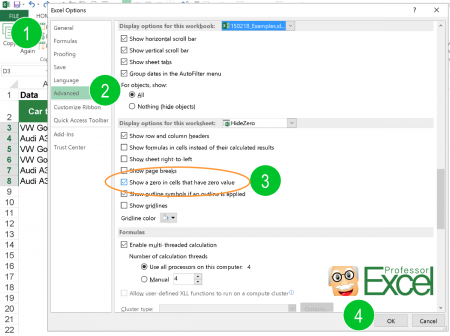
Probably the easiest option is to just not display 0 values. You could differentiate if you want to hide all zeroes from the entire worksheet or just from selected cells.
There are three methods of hiding zero values.
- Hide zero values with conditional formatting rules.
- Blind out zeros with a custom number format.
- Hide zero values within the worksheet settings.
For details about all three methods of just hiding zeroes, please refer to this article.

One small advice on my own account: My Excel add-in “Professor Excel Tools” has a built-in Layout Manager. With this, you can apply this formatting easily to a complete Excel workbook.
Give it a try? Click here and the download starts right away.
Option 2: Change zeroes to blank cells
Unlike the first option, the second option changes the output value. No matter if the return value is 0 (zero) or originally a blank cell, the output of the formula is an empty cell. You can achieve this using the IF formula.
Say, your lookup formula looks like this: =VLOOKUP(A3,C:D,2,FALSE) (hereafter referred to by “original formula”). You want to prevent getting a zero even if the return value―found by the VLOOKUP formula in column D―is an empty value. This can be achieved using the IF formula.
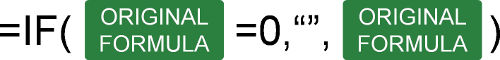
The structure of such IF formula is shown in the image above (if you need assistance with the IF formula, please refer to this article). The original formula is wrapped within the IF formula. The first argument compares if the original formula returns 0. If yes―and that’s the task of the second argument―the formula returns nothing through the double quotation marks. If the orgininal formula within the first argument doesn’t return zero, the last argument returns the real value. This is achieved by the original formula again.
The complete formula looks like this.
=IF(VLOOKUP(A3,C:D,2,FALSE)=0,"",VLOOKUP(A3,C:D,2,FALSE))
Do you want to boost your productivity in Excel?
Get the Professor Excel ribbon!

Add more than 120 great features to Excel!
Option 3: Show zeroes but don’t show blank or empty return values
The previous option two didn’t differentiate between 0 and empty cells in the return cell. If you only want to show empty cells if the return cell found by your lookup formula is empty (and not if the return value really is 0) then you have to slightly alter the formula from option 2 before.
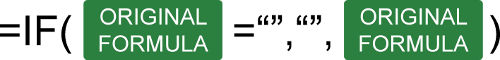
Like before, the IF formula is wrapped around the original formula. But instead of testing if the return value is 0, it tests within the first argument if the return value is blank. This is done by the double quotation marks. The rest of the formula is the as before: With the second argument you define that—if the value from the original formula is blank—the return value is empty too. If not, the last argument defines that you return the desired non-blank value.
The formula in your example from option 2 looks like this.
=IF(VLOOKUP(A3,C:D,2,FALSE)="","",VLOOKUP(A3,C:D,2,FALSE))
Option 4: Use Professor Excel Tools to insert the IF functions very quickly
To save some time, we have included a feature for showing blank cells (instead of zeros) in our Excel add-in Professor Excel Tools.
It’s very simple:
- Select the cells that are supposed to return blanks (instead of zeros).
- Click on the arrow under the “Return Blanks” button on the Professor Excel ribbon and then on either
- Return blanks for zeros and blanks or
- Return zeros for zeros and blanks for blanks.
Professor Excel then inserts the IF function as shown in options 2 and 3 above.

This function is included in our Excel Add-In ‘Professor Excel Tools’
(No sign-up, download starts directly)
Option 5: One elegant solution for not returning zero values…
… was written in the comments. Thanks, Dom! Great to get such awesome feedback from you!
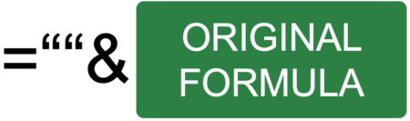
It’s actually quite straight forward: Add two quotation marks in front or after the function and concatenate it with the “&”-character. So, in this case the VLOOKUP function from above would look like this:
=""&VLOOKUP(A3,C:D,2,FALSE)
But: There is a downside. This method forces the cell to a text / string value. This might cause problems in further calculations if a zero is returned. Let me give you an example:
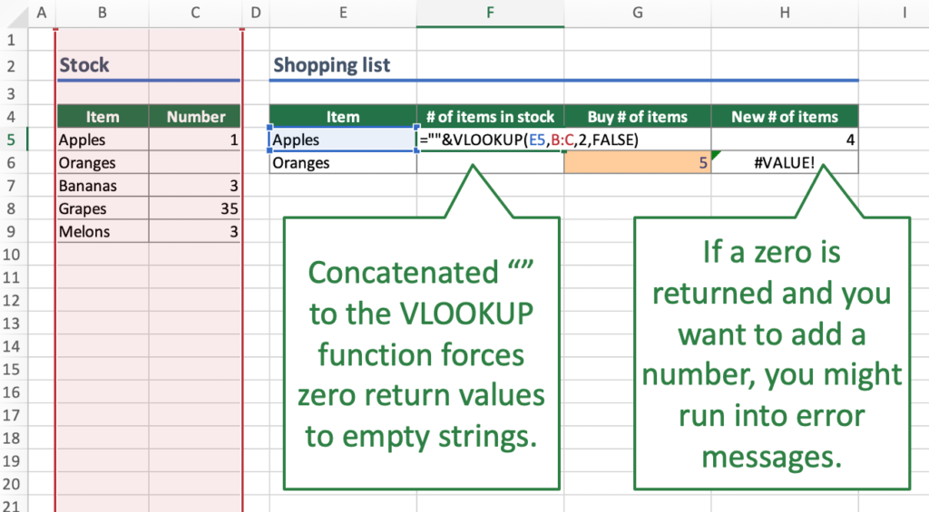
Careful: Return value is interpretated as text.Your VLOOKUP function above is concatenated to an empty string “”. If your return value is 0, the cell will be shown as an empty string. Further calculations might be difficult: For example, if you want to add a number to the return value. Referring directly to the cell, for example =F6+G6 leads to the #VALUE error message as shown above. However, using the SUM function =SUM(F6,G6) still works.
Bottom line: This is an elegant approach, but please test it well if it suits to your Excel model.
Image by Pexels from Pixabay