
An array formula is a formula that can perform multiple calculations on one or more items in an array. You can think of an array as a row or column of values, or a combination of rows and columns of values. Array formulas can return either multiple results, or a single result.
Beginning with the September 2018 update for Microsoft 365, any formula that can return multiple results will automatically spill them either down, or across into neighboring cells. This change in behavior is also accompanied by several new dynamic array functions. Dynamic array formulas, whether they’re using existing functions or the dynamic array functions, only need to be input into a single cell, then confirmed by pressing Enter. Earlier, legacy array formulas require first selecting the entire output range, then confirming the formula with Ctrl+Shift+Enter. They’re commonly referred to as CSE formulas.
You can use array formulas to perform complex tasks, such as:
-
Quickly create sample datasets.
-
Count the number of characters contained in a range of cells.
-
Sum only numbers that meet certain conditions, such as the lowest values in a range, or numbers that fall between an upper and lower boundary.
-
Sum every Nth value in a range of values.
The following examples show you how to create multi-cell and single-cell array formulas. Where possible, we’ve included examples with some of the dynamic array functions, as well as existing array formulas entered as both dynamic and legacy arrays.
Download our examples
Download an example workbook with all the array formula examples in this article.
This exercise shows you how to use multi-cell and single-cell array formulas to calculate a set of sales figures. The first set of steps uses a multi-cell formula to calculate a set of subtotals. The second set uses a single-cell formula to calculate a grand total.
-
Multi-cell array formula

-
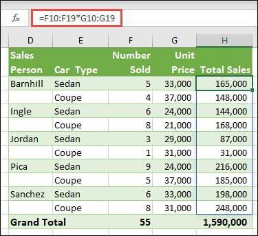
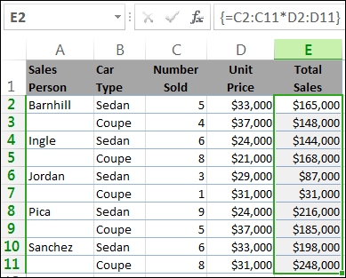
Here we’re calculating Total Sales of coupes and sedans for each salesperson by entering =F10:F19*G10:G19 in cell H10.
When you press Enter, you’ll see the results spill down to cells H10:H19. Notice that the spill range is highlighted with a border when you select any cell within the spill range. You might also notice that the formulas in cells H10:H19 are grayed out. They’re just there for reference, so if you want to adjust the formula, you’ll need to select cell H10, where the master formula lives.
-
Single-cell array formula
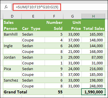
In cell H20 of the example workbook, type or copy and paste =SUM(F10:F19*G10:G19), and then press Enter.
In this case, Excel multiplies the values in the array (the cell range F10 through G19), and then uses the SUM function to add the totals together. The result is a grand total of $1,590,000 in sales.
This example shows how powerful this type of formula can be. For example, suppose you have 1,000 rows of data. You can sum part or all of that data by creating an array formula in a single cell instead of dragging the formula down through the 1,000 rows. Also, notice that the single-cell formula in cell H20 is completely independent of the multi-cell formula (the formula in cells H10 through H19). This is another advantage of using array formulas — flexibility. You could change the other formulas in column H without affecting the formula in H20. It can also be good practice to have independent totals like this, as it helps validate the accuracy of your results.
-
Dynamic array formulas also offer these advantages:
-
Consistency If you click any of the cells from H10 downward, you see the same formula. That consistency can help ensure greater accuracy.
-
Safety You can’t overwrite a component of a multi-cell array formula. For example, click cell H11 and press Delete. Excel won’t change the array’s output. To change it, you need to select the top-left cell in the array, or cell H10.
-
Smaller file sizes You can often use a single array formula instead of several intermediate formulas. For example, the car sales example uses one array formula to calculate the results in column E. If you had used standard formulas such as =F10*G10, F11*G11, F12*G12, etc., you would have used 11 different formulas to calculate the same results. That’s not a big deal, but what if you had thousands of rows to total? Then it can make a big difference.
-
Efficiency Array functions can be an efficient way to build complex formulas. The array formula =SUM(F10:F19*G10:G19) is the same as this: =SUM(F10*G10,F11*G11,F12*G12,F13*G13,F14*G14,F15*G15,F16*G16,F17*G17,F18*G18,F19*G19).
-
Spilling Dynamic array formulas will automatically spill into the output range. If your source data is in an Excel table, then your dynamic array formulas will automatically resize as you add or remove data.
-
#SPILL! error Dynamic arrays introduced the #SPILL! error, which indicates that the intended spill range is blocked for some reason. When you resolve the blockage, the formula will automatically spill.
-
Array constants are a component of array formulas. You create array constants by entering a list of items and then manually surrounding the list with braces ({ }), like this:
={1,2,3,4,5} or ={«January»,»February»,»March»}
If you separate the items by using commas, you create a horizontal array (a row). If you separate the items by using semicolons, you create a vertical array (a column). To create a two-dimensional array, you delimit the items in each row with commas, and delimit each row with semicolons.
The following procedures will give you some practice in creating horizontal, vertical, and two-dimensional constants. We’ll show examples using the SEQUENCE function to automatically generate array constants, as well as manually entered array constants.
-
Create a horizontal constant
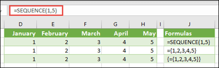
Use the workbook from the previous examples, or create a new workbook. Select any empty cell and enter =SEQUENCE(1,5). The SEQUENCE function builds a 1 row by 5 column array the same as ={1,2,3,4,5}. The following result is displayed:
-
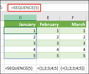
Create a vertical constant
Select any blank cell with room beneath it, and enter =SEQUENCE(5), or ={1;2;3;4;5}. The following result is displayed:
-
Create a two-dimensional constant
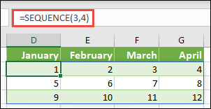
Select any blank cell with room to the right and beneath it, and enter =SEQUENCE(3,4). You see the following result:
You can also enter: or ={1,2,3,4;5,6,7,8;9,10,11,12}, but you’ll want to pay attention to where you put semi-colons versus commas.
As you can see, the SEQUENCE option offers significant advantages over manually entering your array constant values. Primarily, it saves you time, but it can also help reduce errors from manual entry. It’s also easier to read, especially as the semi-colons can be hard to distinguish from the comma separators.
Here’s an example that uses array constants as part of a bigger formula. In the sample workbook, go to the Constant in a formula worksheet, or create a new worksheet.
In cell D9, we entered =SEQUENCE(1,5,3,1), but you could also enter 3, 4, 5, 6, and 7 in cells A9:H9. There’s nothing special about that particular number selection, we just chose something other than 1-5 for differentiation.
In cell E11, enter =SUM(D9:H9*SEQUENCE(1,5)), or =SUM(D9:H9*{1,2,3,4,5}). The formulas return 85.
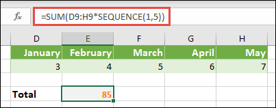
The SEQUENCE function builds the equivalent of the array constant {1,2,3,4,5}. Because Excel performs operations on expressions enclosed in parentheses first, the next two elements that come into play are the cell values in D9:H9, and the multiplication operator (*). At this point, the formula multiplies the values in the stored array by the corresponding values in the constant. It’s the equivalent of:
=SUM(D9*1,E9*2,F9*3,G9*4,H9*5), or =SUM(3*1,4*2,5*3,6*4,7*5)
Finally, the SUM function adds the values, and returns 85.
To avoid using the stored array and keep the operation entirely in memory, you can replace it with another array constant:
=SUM(SEQUENCE(1,5,3,1)*SEQUENCE(1,5)), or =SUM({3,4,5,6,7}*{1,2,3,4,5})
Elements that you can use in array constants
-
Array constants can contain numbers, text, logical values (such as TRUE and FALSE), and error values such as #N/A. You can use numbers in integer, decimal, and scientific formats. If you include text, you need to surround it with quotation marks («text”).
-
Array constants can’t contain additional arrays, formulas, or functions. In other words, they can contain only text or numbers that are separated by commas or semicolons. Excel displays a warning message when you enter a formula such as {1,2,A1:D4} or {1,2,SUM(Q2:Z8)}. Also, numeric values can’t contain percent signs, dollar signs, commas, or parentheses.
One of the best ways to use array constants is to name them. Named constants can be much easier to use, and they can hide some of the complexity of your array formulas from others. To name an array constant and use it in a formula, do the following:
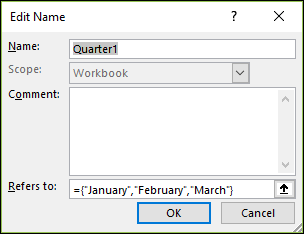
Go to Formulas > Defined Names > Define Name. In the Name box, type Quarter1. In the Refers to box, enter the following constant (remember to type the braces manually):
={«January»,»February»,»March»}
The dialog box should now look like this:
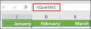
Click OK, then select any row with three blank cells, and enter =Quarter1.
The following result is displayed:
If you want the results to spill vertically instead of horizontally, you can use =TRANSPOSE(Quarter1).
If you want to display a list of 12 months, like you might use when building a financial statement, you can base one off the current year with the SEQUENCE function. The neat thing about this function is that even though only the month is displaying, there is a valid date behind it that you can use in other calculations. You’ll find these examples on the Named array constant and Quick sample dataset worksheets in the example workbook.
=TEXT(DATE(YEAR(TODAY()),SEQUENCE(1,12),1),»mmm»)
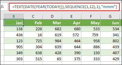
This uses the DATE function to create a date based on the current year, SEQUENCE creates an array constant from 1 to 12 for January through December, then the TEXT function converts the display format to «mmm» (Jan, Feb, Mar, etc.). If you wanted to display the full month name, such as January, you’d use «mmmm».
When you use a named constant as an array formula, remember to enter the equal sign, as in =Quarter1, not just Quarter1. If you don’t, Excel interprets the array as a string of text and your formula won’t work as expected. Finally, keep in mind that you can use combinations of functions, text and numbers. It all depends on how creative you want to get.
The following examples demonstrate a few of the ways in which you can put array constants to use in array formulas. Some of the examples use the TRANSPOSE function to convert rows to columns and vice versa.
-
Multiple each item in an array
Enter =SEQUENCE(1,12)*2, or ={1,2,3,4;5,6,7,8;9,10,11,12}*2
You can also divide with (/), add with (+), and subtract with (—).
-
Square the items in an array
Enter =SEQUENCE(1,12)^2, or ={1,2,3,4;5,6,7,8;9,10,11,12}^2
-
Find the square root of squared items in an array
Enter =SQRT(SEQUENCE(1,12)^2), or =SQRT({1,2,3,4;5,6,7,8;9,10,11,12}^2)
-
Transpose a one-dimensional row
Enter =TRANSPOSE(SEQUENCE(1,5)), or =TRANSPOSE({1,2,3,4,5})
Even though you entered a horizontal array constant, the TRANSPOSE function converts the array constant into a column.
-
Transpose a one-dimensional column
Enter =TRANSPOSE(SEQUENCE(5,1)), or =TRANSPOSE({1;2;3;4;5})
Even though you entered a vertical array constant, the TRANSPOSE function converts the constant into a row.
-
Transpose a two-dimensional constant
Enter =TRANSPOSE(SEQUENCE(3,4)), or =TRANSPOSE({1,2,3,4;5,6,7,8;9,10,11,12})
The TRANSPOSE function converts each row into a series of columns.
This section provides examples of basic array formulas.
-
Create an array from existing values
The following example explains how to use array formulas to create a new array from an existing array.
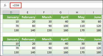
Enter =SEQUENCE(3,6,10,10), or ={10,20,30,40,50,60;70,80,90,100,110,120;130,140,150,160,170,180}
Be sure to type { (opening brace) before you type 10, and } (closing brace) after you type 180, because you’re creating an array of numbers.
Next, enter =D9#, or =D9:I11 in a blank cell. A 3 x 6 array of cells appears with the same values you see in D9:D11. The # sign is called the spilled range operator, and it’s Excel’s way of referencing the entire array range instead of having to type it out.
-
Create an array constant from existing values
You can take the results of a spilled array formula and convert that into its component parts. Select cell D9, then press F2 to switch to edit mode. Next, press F9 to convert the cell references to values, which Excel then converts into an array constant. When you press Enter, the formula, =D9#, should now be ={10,20,30;40,50,60;70,80,90}.
-
Count characters in a range of cells
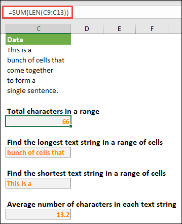
The following example shows you how to count the number of characters in a range of cells. This includes spaces.
=SUM(LEN(C9:C13))
In this case, the LEN function returns the length of each text string in each of the cells in the range. The SUM function then adds those values together and displays the result (66). If you wanted to get average number of characters, you could use:
=AVERAGE(LEN(C9:C13))
-
Contents of longest cell in range C9:C13
=INDEX(C9:C13,MATCH(MAX(LEN(C9:C13)),LEN(C9:C13),0),1)
This formula works only when a data range contains a single column of cells.
Let’s take a closer look at the formula, starting from the inner elements and working outward. The LEN function returns the length of each of the items in the cell range D2:D6. The MAX function calculates the largest value among those items, which corresponds to the longest text string, which is in cell D3.
Here’s where things get a little complex. The MATCH function calculates the offset (the relative position) of the cell that contains the longest text string. To do that, it requires three arguments: a lookup value, a lookup array, and a match type. The MATCH function searches the lookup array for the specified lookup value. In this case, the lookup value is the longest text string:
MAX(LEN(C9:C13)
and that string resides in this array:
LEN(C9:C13)
The match type argument in this case is 0. The match type can be a 1, 0, or -1 value.
-
1 — returns the largest value that is less than or equal to the lookup val
-
0 — returns the first value exactly equal to the lookup value
-
-1 — returns the smallest value that is greater than or equal to the specified lookup value
-
If you omit a match type, Excel assumes 1.
Finally, the INDEX function takes these arguments: an array, and a row and column number within that array. The cell range C9:C13 provides the array, the MATCH function provides the cell address, and the final argument (1) specifies that the value comes from the first column in the array.
If you wanted to get the contents of the smallest text string, you would replace MAX in the above example with MIN.
-
-
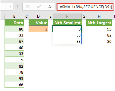
Find the n smallest values in a range
This example shows how to find the three smallest values in a range of cells, where an array of sample data in cells B9:B18has been created with: =INT(RANDARRAY(10,1)*100). Note that RANDARRAY is a volatile function, so you’ll get a new set of random numbers each time Excel calculates.
Enter =SMALL(B9#,SEQUENCE(D9), =SMALL(B9:B18,{1;2;3})
This formula uses an array constant to evaluate the SMALL function three times and return the smallest 3 members in the array that’s contained in cells B9:B18, where 3 is a variable value in cell D9. To find more values, you can increase the value in the SEQUENCE function, or add more arguments to the constant. You can also use additional functions with this formula, such as SUM or AVERAGE. For example:
=SUM(SMALL(B9#,SEQUENCE(D9))
=AVERAGE(SMALL(B9#,SEQUENCE(D9))
-
Find the n largest values in a range
To find the largest values in a range, you can replace the SMALL function with the LARGE function. In addition, the following example uses the ROW and INDIRECT functions.
Enter =LARGE(B9#,ROW(INDIRECT(«1:3»))), or =LARGE(B9:B18,ROW(INDIRECT(«1:3»)))
At this point, it may help to know a bit about the ROW and INDIRECT functions. You can use the ROW function to create an array of consecutive integers. For example, select an empty and enter:
=ROW(1:10)
The formula creates a column of 10 consecutive integers. To see a potential problem, insert a row above the range that contains the array formula (that is, above row 1). Excel adjusts the row references, and the formula now generates integers from 2 to 11. To fix that problem, you add the INDIRECT function to the formula:
=ROW(INDIRECT(«1:10»))
The INDIRECT function uses text strings as its arguments (which is why the range 1:10 is surrounded by quotation marks). Excel does not adjust text values when you insert rows or otherwise move the array formula. As a result, the ROW function always generates the array of integers that you want. You could just as easily use SEQUENCE:
=SEQUENCE(10)
Let’s examine the formula that you used earlier — =LARGE(B9#,ROW(INDIRECT(«1:3»))) — starting from the inner parentheses and working outward: The INDIRECT function returns a set of text values, in this case the values 1 through 3. The ROW function in turn generates a three-cell column array. The LARGE function uses the values in the cell range B9:B18, and it is evaluated three times, once for each reference returned by the ROW function. If you want to find more values, you add a greater cell range to the INDIRECT function. Finally, as with the SMALL examples, you can use this formula with other functions, such as SUM and AVERAGE.
-
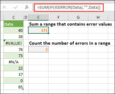
Sum a range that contains error values
The SUM function in Excel does not work when you try to sum a range that contains an error value, such as #VALUE! or #N/A. This example shows you how to sum the values in a range named Data that contains errors:
-
=SUM(IF(ISERROR(Data),»»,Data))
The formula creates a new array that contains the original values minus any error values. Starting from the inner functions and working outward, the ISERROR function searches the cell range (Data) for errors. The IF function returns a specific value if a condition you specify evaluates to TRUE and another value if it evaluates to FALSE. In this case, it returns empty strings («») for all error values because they evaluate to TRUE, and it returns the remaining values from the range (Data) because they evaluate to FALSE, meaning that they don’t contain error values. The SUM function then calculates the total for the filtered array.
-
Count the number of error values in a range
This example is like the previous formula, but it returns the number of error values in a range named Data instead of filtering them out:
=SUM(IF(ISERROR(Data),1,0))
This formula creates an array that contains the value 1 for the cells that contain errors and the value 0 for the cells that don’t contain errors. You can simplify the formula and achieve the same result by removing the third argument for the IF function, like this:
=SUM(IF(ISERROR(Data),1))
If you don’t specify the argument, the IF function returns FALSE if a cell does not contain an error value. You can simplify the formula even more:
=SUM(IF(ISERROR(Data)*1))
This version works because TRUE*1=1 and FALSE*1=0.
You might need to sum values based on conditions.
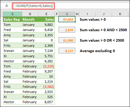
For example, this array formula sums just the positive integers in a range named Sales, which represents cells E9:E24 in the example above:
=SUM(IF(Sales>0,Sales))
The IF function creates an array of positive and false values. The SUM function essentially ignores the false values because 0+0=0. The cell range that you use in this formula can consist of any number of rows and columns.
You can also sum values that meet more than one condition. For example, this array formula calculates values greater than 0 AND less than 2500:
=SUM((Sales>0)*(Sales<2500)*(Sales))
Keep in mind that this formula returns an error if the range contains one or more non-numeric cells.
You can also create array formulas that use a type of OR condition. For example, you can sum values that are greater than 0 OR less than 2500:
=SUM(IF((Sales>0)+(Sales<2500),Sales))
You can’t use the AND and OR functions in array formulas directly because those functions return a single result, either TRUE or FALSE, and array functions require arrays of results. You can work around the problem by using the logic shown in the previous formula. In other words, you perform math operations, such as addition or multiplication on values that meet the OR or AND condition.
This example shows you how to remove zeros from a range when you need to average the values in that range. The formula uses a data range named Sales:
=AVERAGE(IF(Sales<>0,Sales))
The IF function creates an array of values that do not equal 0 and then passes those values to the AVERAGE function.
This array formula compares the values in two ranges of cells named MyData and YourData and returns the number of differences between the two. If the contents of the two ranges are identical, the formula returns 0. To use this formula, the cell ranges need to be the same size and of the same dimension. For example, if MyData is a range of 3 rows by 5 columns, YourData must also be 3 rows by 5 columns:
=SUM(IF(MyData=YourData,0,1))
The formula creates a new array of the same size as the ranges that you are comparing. The IF function fills the array with the value 0 and the value 1 (0 for mismatches and 1 for identical cells). The SUM function then returns the sum of the values in the array.
You can simplify the formula like this:
=SUM(1*(MyData<>YourData))
Like the formula that counts error values in a range, this formula works because TRUE*1=1, and FALSE*1=0.
This array formula returns the row number of the maximum value in a single-column range named Data:
=MIN(IF(Data=MAX(Data),ROW(Data),»»))
The IF function creates a new array that corresponds to the range named Data. If a corresponding cell contains the maximum value in the range, the array contains the row number. Otherwise, the array contains an empty string («»). The MIN function uses the new array as its second argument and returns the smallest value, which corresponds to the row number of the maximum value in Data. If the range named Data contains identical maximum values, the formula returns the row of the first value.
If you want to return the actual cell address of a maximum value, use this formula:
=ADDRESS(MIN(IF(Data=MAX(Data),ROW(Data),»»)),COLUMN(Data))
You’ll find similar examples in the sample workbook on the Differences between datasets worksheet.
This exercise shows you how to use multi-cell and single-cell array formulas to calculate a set of sales figures. The first set of steps uses a multi-cell formula to calculate a set of subtotals. The second set uses a single-cell formula to calculate a grand total.
-
Multi-cell array formula
Copy the entire table below and paste it into cell A1 in a blank worksheet.
|
Sales |
Car |
Number |
Unit |
Total |
|---|---|---|---|---|
|
Barnhill |
Sedan |
5 |
33000 |
|
|
Coupe |
4 |
37000 |
||
|
Ingle |
Sedan |
6 |
24000 |
|
|
Coupe |
8 |
21000 |
||
|
Jordan |
Sedan |
3 |
29000 |
|
|
Coupe |
1 |
31000 |
||
|
Pica |
Sedan |
9 |
24000 |
|
|
Coupe |
5 |
37000 |
||
|
Sanchez |
Sedan |
6 |
33000 |
|
|
Coupe |
8 |
31000 |
||
|
Formula (Grand Total) |
Grand Total |
|||
|
‘=SUM(C2:C11*D2:D11) |
=SUM(C2:C11*D2:D11) |
-
To see Total Sales of coupes and sedans for each salesperson, select cells E2:E11, enter the formula =C2:C11*D2:D11, and then press Ctrl+Shift+Enter.
-
To see the Grand Total of all sales, select cell F11, enter the formula =SUM(C2:C11*D2:D11), and then press Ctrl+Shift+Enter.
When you press Ctrl+Shift+Enter, Excel surrounds the formula with braces ({ }) and inserts an instance of the formula in each cell of the selected range. This happens very quickly, so what you see in column E is the total sales amount for each car type for each salesperson. If you select E2, then select E3, E4, and so on, you’ll see that the same formula is shown: {=C2:C11*D2:D11}.
-
Create a single-cell array formula
In cell D13 of the workbook, type the following formula, and then press Ctrl+Shift+Enter:
=SUM(C2:C11*D2:D11)
In this case, Excel multiplies the values in the array (the cell range C2 through D11) and then uses the SUM function to add the totals together. The result is a grand total of $1,590,000 in sales. This example shows how powerful this type of formula can be. For example, suppose you have 1,000 rows of data. You can sum part or all of that data by creating an array formula in a single cell instead of dragging the formula down through the 1,000 rows.
Also, notice that the single-cell formula in cell D13 is completely independent of the multi-cell formula (the formula in cells E2 through E11). This is another advantage of using array formulas — flexibility. You could change the formulas in column E or delete that column altogether, without affecting the formula in D13.
Array formulas also offer these advantages:
-
Consistency If you click any of the cells from E2 downward, you see the same formula. That consistency can help ensure greater accuracy.
-
Safety You cannot overwrite a component of a multi-cell array formula. For example, click cell E3 and press Delete. You have to either select the entire range of cells (E2 through E11) and change the formula for the entire array, or leave the array as is. As an added safety measure, you have to press Ctrl+Shift+Enter to confirm any change to the formula.
-
Smaller file sizes You can often use a single array formula instead of several intermediate formulas. For example, the workbook uses one array formula to calculate the results in column E. If you had used standard formulas (such as =C2*D2, C3*D3, C4*D4…), you would have used 11 different formulas to calculate the same results.
In general, array formulas use standard formula syntax. They all begin with an equal (=) sign, and you can use most of the built-in Excel functions in your array formulas. The key difference is that when using an array formula, you press Ctrl+Shift+Enter to enter your formula. When you do this, Excel surrounds your array formula with braces — if you type the braces manually, your formula will be converted to a text string, and it won’t work.
Array functions can be an efficient way to build complex formulas. The array formula =SUM(C2:C11*D2:D11) is the same as this: =SUM(C2*D2,C3*D3,C4*D4,C5*D5,C6*D6,C7*D7,C8*D8,C9*D9,C10*D10,C11*D11).
Important: Press Ctrl+Shift+Enter whenever you need to enter an array formula. This applies to both single-cell and multi-cell formulas.
Whenever you work with multi-cell formulas, also remember:
-
Select the range of cells to hold your results before you enter the formula. You did this when you created the multi-cell array formula when you selected cells E2 through E11.
-
You can’t change the contents of an individual cell in an array formula. To try this, select cell E3 in the workbook and press Delete. Excel displays a message that tells you that you can’t change part of an array.
-
You can move or delete an entire array formula, but you can’t move or delete part of it. In other words, to shrink an array formula, you first delete the existing formula and then start over.
-
To delete an array formula, select the entire formula range (for example, E2:E11), then press Delete.
-
You can’t insert blank cells into, or delete cells from a multi-cell array formula.
At times, you may need to expand an array formula. Select the first cell in existing array range, and continue until you’ve selected the entire range that you want to extend the formula to. Press F2 to edit the formula, then press CTRL+SHIFT+ENTER to confirm the formula once you’ve adjusted the formula range. The key is to select the entire range, starting with the top-left cell in the array. The top-left cell is the one that gets edited.
Array formulas are great, but they can have some disadvantages:
-
You may occasionally forget to press Ctrl+Shift+Enter. It can happen to even the most experienced Excel users. Remember to press this key combination whenever you enter or edit an array formula.
-
Other users of your workbook might not understand your formulas. In practice, array formulas are generally not explained in a worksheet. Therefore, if other people need to modify your workbooks, you should either avoid array formulas or make sure those people know about any array formulas and understand how to change them, if they need to.
-
Depending on the processing speed and memory of your computer, large array formulas can slow down calculations.
Array constants are a component of array formulas. You create array constants by entering a list of items and then manually surrounding the list with braces ({ }), like this:
={1,2,3,4,5}
By now, you know you need to press Ctrl+Shift+Enter when you create array formulas. Because array constants are a component of array formulas, you surround the constants with braces by manually typing them. You then use Ctrl+Shift+Enter to enter the entire formula.
If you separate the items by using commas, you create a horizontal array (a row). If you separate the items by using semicolons, you create a vertical array (a column). To create a two-dimensional array, you delimit the items in each row by using commas and delimit each row by using semicolons.
Here’s an array in a single row: {1,2,3,4}. Here’s an array in a single column: {1;2;3;4}. And here’s an array of two rows and four columns: {1,2,3,4;5,6,7,8}. In the two row array, the first row is 1, 2, 3, and 4, and the second row is 5, 6, 7, and 8. A single semicolon separates the two rows, between 4 and 5.
As with array formulas, you can use array constants with most of the built-in functions that Excel provides. The following sections explain how to create each kind of constant and how to use these constants with functions in Excel.
The following procedures will give you some practice in creating horizontal, vertical, and two-dimensional constants.
Create a horizontal constant
-
In a blank worksheet, select cells A1 through E1.
-
In the formula bar, enter the following formula, and then press Ctrl+Shift+Enter:
={1,2,3,4,5}
In this case, you should type the opening and closing braces ({ }), and Excel will add the second set for you.
The following result is displayed.
Create a vertical constant
-
In your workbook, select a column of five cells.
-
In the formula bar, enter the following formula, and then press Ctrl+Shift+Enter:
={1;2;3;4;5}
The following result is displayed.
Create a two-dimensional constant
-
In your workbook, select a block of cells four columns wide by three rows high.
-
In the formula bar, enter the following formula, and then press Ctrl+Shift+Enter:
={1,2,3,4;5,6,7,8;9,10,11,12}
You see the following result:
Use constants in formulas
Here is a simple example that uses constants:
-
In the sample workbook, create a new worksheet.
-
In cell A1, type 3, and then type 4 in B1, 5 in C1, 6 in D1, and 7 in E1.
-
In cell A3, type the following formula, and then press Ctrl+Shift+Enter:
=SUM(A1:E1*{1,2,3,4,5})
Notice that Excel surrounds the constant with another set of braces, because you entered it as an array formula.
The value 85 appears in cell A3.
The next section explains how the formula works.
The formula you just used contains several parts.
1. Function
2. Stored array
3. Operator
4. Array constant
The last element inside the parentheses is the array constant: {1,2,3,4,5}. Remember that Excel does not surround array constants with braces; you actually type them. Also remember that after you add a constant to an array formula, you press Ctrl+Shift+Enter to enter the formula.
Because Excel performs operations on expressions enclosed in parentheses first, the next two elements that come into play are the values stored in the workbook (A1:E1) and the operator. At this point, the formula multiplies the values in the stored array by the corresponding values in the constant. It’s the equivalent of:
=SUM(A1*1,B1*2,C1*3,D1*4,E1*5)
Finally, the SUM function adds the values, and the sum 85 appears in cell A3.
To avoid using the stored array and to just keep the operation entirely in memory, replace the stored array with another array constant:
=SUM({3,4,5,6,7}*{1,2,3,4,5})
To try this, copy the function, select a blank cell in your workbook, paste the formula into the formula bar, and then press Ctrl+Shift+Enter. You’ll see the same result as you did in the earlier exercise that used the array formula:
=SUM(A1:E1*{1,2,3,4,5})
Array constants can contain numbers, text, logical values (such as TRUE and FALSE), and error values ( such as #N/A). You can use numbers in the integer, decimal, and scientific formats. If you include text, you need to surround the text with quotation marks («).
Array constants can’t contain additional arrays, formulas, or functions. In other words, they can contain only text or numbers that are separated by commas or semicolons. Excel displays a warning message when you enter a formula such as {1,2,A1:D4} or {1,2,SUM(Q2:Z8)}. Also, numeric values can’t contain percent signs, dollar signs, commas, or parentheses.
One of the best way to use array constants is to name them. Named constants can be much easier to use, and they can hide some of the complexity of your array formulas from others. To name an array constant and use it in a formula, do the following:
-
On the Formulas tab, in the Defined Names group, click Define Name.
The Define Name dialog box appears. -
In the Name box, type Quarter1.
-
In the Refers to box, enter the following constant (remember to type the braces manually):
={«January»,»February»,»March»}
The contents of the dialog box now looks like this:
-
Click OK, and then select a row of three blank cells.
-
Type the following formula, and then press Ctrl+Shift+Enter.
=Quarter1
The following result is displayed.
When you use a named constant as an array formula, remember to enter the equal sign. If you don’t, Excel interprets the array as a string of text and your formula won’t work as expected. Finally, keep in mind that you can use combinations of text and numbers.
Look for the following problems when your array constants don’t work:
-
Some elements might not be separated with the proper character. If you omit a comma or semicolon, or if you put one in the wrong place, the array constant might not be created correctly, or you might see a warning message.
-
You might have selected a range of cells that doesn’t match the number of elements in your constant. For example, if you select a column of six cells for use with a five-cell constant, the #N/A error value appears in the empty cell. Conversely, if you select too few cells, Excel omits the values that don’t have a corresponding cell.
The following examples demonstrate a few of the ways in which you can put array constants to use in array formulas. Some of the examples use the TRANSPOSE function to convert rows to columns and vice versa.
Multiply each item in an array
-
Create a new worksheet, and then select a block of empty cells four columns wide by three rows high.
-
Type the following formula, and then press Ctrl+Shift+Enter:
={1,2,3,4;5,6,7,8;9,10,11,12}*2
Square the items in an array
-
Select a block of empty cells four columns wide by three rows high.
-
Type the following array formula, and then press Ctrl+Shift+Enter:
={1,2,3,4;5,6,7,8;9,10,11,12}*{1,2,3,4;5,6,7,8;9,10,11,12}
Alternatively, enter this array formula, which uses the caret operator (^):
={1,2,3,4;5,6,7,8;9,10,11,12}^2
Transpose a one-dimensional row
-
Select a column of five blank cells.
-
Type the following formula, and then press Ctrl+Shift+Enter:
=TRANSPOSE({1,2,3,4,5})
Even though you entered a horizontal array constant, the TRANSPOSE function converts the array constant into a column.
Transpose a one-dimensional column
-
Select a row of five blank cells.
-
Enter the following formula, and then press Ctrl+Shift+Enter:
=TRANSPOSE({1;2;3;4;5})
Even though you entered a vertical array constant, the TRANSPOSE function converts the constant into a row.
Transpose a two-dimensional constant
-
Select a block of cells three columns wide by four rows high.
-
Enter the following constant, and then press Ctrl+Shift+Enter:
=TRANSPOSE({1,2,3,4;5,6,7,8;9,10,11,12})
The TRANSPOSE function converts each row into a series of columns.
This section provides examples of basic array formulas.
Create arrays and array constants from existing values
The following example explains how to use array formulas to create links between ranges of cells in different worksheets. It also shows you how to create an array constant from the same set of values.
Create an array from existing values
-
On a worksheet in Excel, select cells C8:E10, and enter this formula:
={10,20,30;40,50,60;70,80,90}
Be sure to type { (opening brace) before you type 10, and } (closing brace) after you type 90, because you’re creating an array of numbers.
-
Press Ctrl+Shift+Enter, which enters this array of numbers in the cell range C8:E10 by using an array formula. On your worksheet, C8 through E10 should look like this:
10
20
30
40
50
60
70
80
90
-
Select the cell range C1 through E3.
-
Enter the following formula in the formula bar, and then press Ctrl+Shift+Enter:
=C8:E10
A 3×3 array of cells appears in cells C1 through E3 with the same values you see in C8 through E10.
Create an array constant from existing values
-
With cells C1:C3 selected, press F2 to switch to edit mode.
-
Press F9 to convert the cell references to values. Excel converts the values into an array constant. The formula should now be ={10,20,30;40,50,60;70,80,90}.
-
Press Ctrl+Shift+Enter to enter the array constant as an array formula.
Count characters in a range of cells
The following example shows you how to count the number of characters, including spaces, in a range of cells.
-
Copy this entire table and paste into a worksheet in cell A1.
Data
This is a
bunch of cells that
come together
to form a
single sentence.
Total characters in A2:A6
=SUM(LEN(A2:A6))
Contents of longest cell (A3)
=INDEX(A2:A6,MATCH(MAX(LEN(A2:A6)),LEN(A2:A6),0),1)
-
Select cell A8, and then press Ctrl+Shift+Enter to see the total number of characters in cells A2:A6 (66).
-
Select cell A10, and then press Ctrl+Shift+Enter to see the contents of the longest of cells A2:A6 (cell A3).
The following formula is used in cell A8 counts the total number of characters (66) in cells A2 through A6.
=SUM(LEN(A2:A6))
In this case, the LEN function returns the length of each text string in each of the cells in the range. The SUM function then adds those values together and displays the result (66).
Find the n smallest values in a range
This example shows how to find the three smallest values in a range of cells.
-
Enter some random numbers in cells A1:A11.
-
Select cells C1 through C3. This set of cells will hold the results returned by the array formula.
-
Enter the following formula, and then press Ctrl+Shift+Enter:
=SMALL(A1:A11,{1;2;3})
This formula uses an array constant to evaluate the SMALL function three times and return the smallest (1), second smallest (2), and third smallest (3) members in the array that is contained in cells A1:A10 To find more values, you add more arguments to the constant. You can also use additional functions with this formula, such as SUM or AVERAGE. For example:
=SUM(SMALL(A1:A10,{1,2,3})
=AVERAGE(SMALL(A1:A10,{1,2,3})
Find the n largest values in a range
To find the largest values in a range, you can replace the SMALL function with the LARGE function. In addition, the following example uses the ROW and INDIRECT functions.
-
Select cells D1 through D3.
-
In the formula bar, enter this formula, and then press Ctrl+Shift+Enter:
=LARGE(A1:A10,ROW(INDIRECT(«1:3»)))
At this point, it may help to know a bit about the ROW and INDIRECT functions. You can use the ROW function to create an array of consecutive integers. For example, select an empty column of 10 cells in your practice workbook, enter this array formula, and then press Ctrl+Shift+Enter:
=ROW(1:10)
The formula creates a column of 10 consecutive integers. To see a potential problem, insert a row above the range that contains the array formula (that is, above row 1). Excel adjusts the row references, and the formula generates integers from 2 to 11. To fix that problem, you add the INDIRECT function to the formula:
=ROW(INDIRECT(«1:10»))
The INDIRECT function uses text strings as its arguments (which is why the range 1:10 is surrounded by double quotation marks). Excel does not adjust text values when you insert rows or otherwise move the array formula. As a result, the ROW function always generates the array of integers that you want.
Let’s take a look at the formula that you used earlier — =LARGE(A5:A14,ROW(INDIRECT(«1:3»))) — starting from the inner parentheses and working outward: The INDIRECT function returns a set of text values, in this case the values 1 through 3. The ROW function in turn generates a three-cell columnar array. The LARGE function uses the values in the cell range A5:A14, and it is evaluated three times, once for each reference returned by the ROW function. The values 3200, 2700, and 2000 are returned to the three-cell columnar array. If you want to find more values, you add a greater cell range to the INDIRECT function.
As with earlier examples, you can use this formula with other functions, such as SUM and AVERAGE.
Find the longest text string in a range of cells
Go back to the earlier text string example, enter the following formula in an empty cell, and press Ctrl+Shift+Enter:
=INDEX(A2:A6,MATCH(MAX(LEN(A2:A6)),LEN(A2:A6),0),1)
The text «bunch of cells that» appears.
Let’s take a closer look at the formula, starting from the inner elements and working outward. The LEN function returns the length of each of the items in the cell range A2:A6. The MAX function calculates the largest value among those items, which corresponds to the longest text string, which is in cell A3.
Here’s where things get a little complex. The MATCH function calculates the offset (the relative position) of the cell that contains the longest text string. To do that, it requires three arguments: a lookup value, a lookup array, and a match type. The MATCH function searches the lookup array for the specified lookup value. In this case, the lookup value is the longest text string:
(MAX(LEN(A2:A6))
and that string resides in this array:
LEN(A2:A6)
The match type argument is 0. The match type can consist of a 1, 0, or -1 value. If you specify 1, MATCH returns the largest value that is less than or equal to the lookup value. If you specify 0, MATCH returns the first value exactly equal to the lookup value. If you specify -1, MATCH finds the smallest value that is greater than or equal to the specified lookup value. If you omit a match type, Excel assumes 1.
Finally, the INDEX function takes these arguments: an array, and a row and column number within that array. The cell range A2:A6 provides the array, the MATCH function provides the cell address, and the final argument (1) specifies that the value comes from the first column in the array.
This section provides examples of advanced array formulas.
Sum a range that contains error values
The SUM function in Excel does not work when you try to sum a range that contains an error value, such as #N/A. This example shows you how to sum the values in a range named Data that contains errors.
=SUM(IF(ISERROR(Data),»»,Data))
The formula creates a new array that contains the original values minus any error values. Starting from the inner functions and working outward, the ISERROR function searches the cell range (Data) for errors. The IF function returns a specific value if a condition you specify evaluates to TRUE and another value if it evaluates to FALSE. In this case, it returns empty strings («») for all error values because they evaluate to TRUE, and it returns the remaining values from the range (Data) because they evaluate to FALSE, meaning that they don’t contain error values. The SUM function then calculates the total for the filtered array.
Count the number of error values in a range
This example is similar to the previous formula, but it returns the number of error values in a range named Data instead of filtering them out:
=SUM(IF(ISERROR(Data),1,0))
This formula creates an array that contains the value 1 for the cells that contain errors and the value 0 for the cells that don’t contain errors. You can simplify the formula and achieve the same result by removing the third argument for the IF function, like this:
=SUM(IF(ISERROR(Data),1))
If you don’t specify the argument, the IF function returns FALSE if a cell does not contain an error value. You can simplify the formula even more:
=SUM(IF(ISERROR(Data)*1))
This version works because TRUE*1=1 and FALSE*1=0.
Sum values based on conditions
You might need to sum values based on conditions. For example, this array formula sums just the positive integers in a range named Sales:
=SUM(IF(Sales>0,Sales))
The IF function creates an array of positive values and false values. The SUM function essentially ignores the false values because 0+0=0. The cell range that you use in this formula can consist of any number of rows and columns.
You can also sum values that meet more than one condition. For example, this array formula calculates values greater than 0 and less than or equal to 5:
=SUM((Sales>0)*(Sales<=5)*(Sales))
Keep in mind that this formula returns an error if the range contains one or more non-numeric cells.
You can also create array formulas that use a type of OR condition. For example, you can sum values that are less than 5 and greater than 15:
=SUM(IF((Sales<5)+(Sales>15),Sales))
The IF function finds all values smaller than 5 and greater than 15 and then passes those values to the SUM function.
You can’t use the AND and OR functions in array formulas directly because those functions return a single result, either TRUE or FALSE, and array functions require arrays of results. You can work around the problem by using the logic shown in the previous formula. In other words, you perform math operations, such as addition or multiplication, on values that meet the OR or AND condition.
Compute an average that excludes zeros
This example shows you how to remove zeros from a range when you need to average the values in that range. The formula uses a data range named Sales:
=AVERAGE(IF(Sales<>0,Sales))
The IF function creates an array of values that do not equal 0 and then passes those values to the AVERAGE function.
Count the number of differences between two ranges of cells
This array formula compares the values in two ranges of cells named MyData and YourData and returns the number of differences between the two. If the contents of the two ranges are identical, the formula returns 0. To use this formula, the cell ranges need to be the same size and of the same dimension (for example, if MyData is a range of 3 rows by 5 columns, YourData must also be 3 rows by 5 columns):
=SUM(IF(MyData=YourData,0,1))
The formula creates a new array of the same size as the ranges that you are comparing. The IF function fills the array with the value 0 and the value 1 (0 for mismatches and 1 for identical cells). The SUM function then returns the sum of the values in the array.
You can simplify the formula like this:
=SUM(1*(MyData<>YourData))
Like the formula that counts error values in a range, this formula works because TRUE*1=1, and FALSE*1=0.
Find the location of the maximum value in a range
This array formula returns the row number of the maximum value in a single-column range named Data:
=MIN(IF(Data=MAX(Data),ROW(Data),»»))
The IF function creates a new array that corresponds to the range named Data. If a corresponding cell contains the maximum value in the range, the array contains the row number. Otherwise, the array contains an empty string («»). The MIN function uses the new array as its second argument and returns the smallest value, which corresponds to the row number of the maximum value in Data. If the range named Data contains identical maximum values, the formula returns the row of the first value.
If you want to return the actual cell address of a maximum value, use this formula:
=ADDRESS(MIN(IF(Data=MAX(Data),ROW(Data),»»)),COLUMN(Data))
Acknowledgement
Parts of this article were based on a series of Excel Power User columns written by Colin Wilcox, and adapted from chapters 14 and 15 of Excel 2002 Formulas, a book written by John Walkenbach, a former Excel MVP.
Need more help?
You can always ask an expert in the Excel Tech Community or get support in the Answers community.
See Also
Dynamic arrays and spilled array behavior
Dynamic array formulas vs. legacy CSE array formulas
FILTER function
RANDARRAY function
SEQUENCE function
SORT function
SORTBY function
UNIQUE function
#SPILL! errors in Excel
Implicit intersection operator: @
Overview of formulas
Formulas are the life and blood of Excel spreadsheets. And in most cases, you don’t need the formula in just one cell or a couple of cells.
In most cases, you would need to apply the formula to an entire column (or a large range of cells in a column).
And Excel gives you multiple different ways to do this with a few clicks (or a keyboard shortcut).
Let’s have a look at these methods.
By Double-Clicking on the AutoFill Handle
One of the easiest ways to apply a formula to an entire column is by using this simple mouse double-click trick.
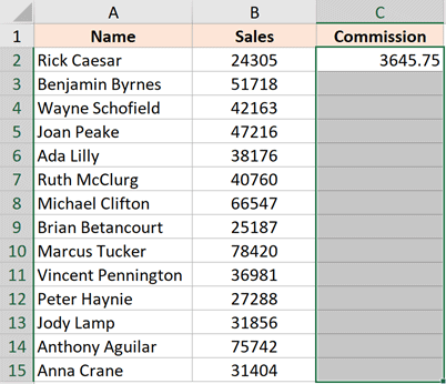
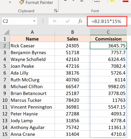
Suppose you have the dataset as shown below, where want to calculate the commission for each sales rep in Column C (where the commission would be 15% of the sale value in column B).
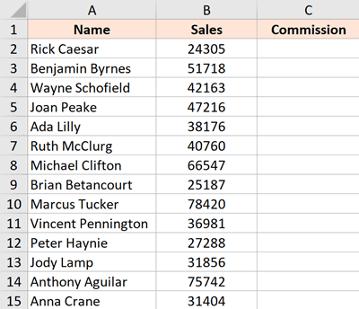
The formula for this would be:
=B2*15%
Below is the way to apply this formula to the entire column C:
- In cell A2, enter the formula: =B2*15%

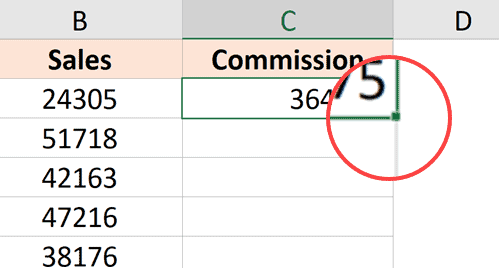
- With the cell selected, you will see a small green square at the bottom-right part of the selection.

- Place the cursor over the small green square. You will notice that the cursor changes to a plus sign (this is called the autofill handle)

- Double click the left mouse key

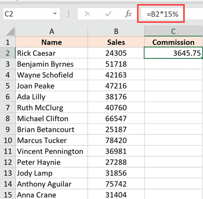
The above steps would automatically fill the entire column till the cell where you have the data in the adjacent column. In our example, the formula would be applied till cell C15
For this to work, there shouldn’t be data in the adjacent column and there should not be any blank cells in it. If, for example, there is a blank cell in column B (say cell B6), then this auto-fill double click would only apply the formula till cell C5
When you use the autofill handle to apply the formula to the entire column, it’s equivalent to copy-pasting the formula manually. This means that the cell reference in the formula would change accordingly.
For example, if it’s an absolute reference, it would remain as is while the formula is applied to the column, add if it’s a relative reference, then it would change as the formula is applied to the cells below.
By Dragging the AutoFill Handle
One issue with the above double click method is that it would stop as soon as it encountered a blank cell in the adjacent columns.
If you have a small data set, you can also manually drag the fill handle to apply the formula in the column.
Below are the steps to do this:
- In cell A2, enter the formula: =B2*15%
- With the cell selected, you will see a small green square at the bottom-right part of the selection
- Place the cursor over the small green square. You will notice that the cursor changes to a plus sign
- Hold the left mouse key and drag it to the cell where you want the formula to be applied
- Leave the mouse key when done
Using the Fill Down Option (it’s in the ribbon)
Another way to apply a formula to the entire column is by using the fill down option in the ribbon.
For this method to work, you first need to select the cells in the column where you want to have the formula.
Below are the steps to use the fill down method:
- In cell A2, enter the formula: =B2*15%
- Select all the cells in which you want to apply the formula (including cell C2)

- Click the Home tab

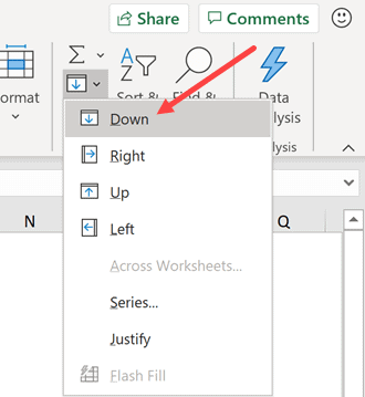
- In the editing group, click on the Fill icon

- Click on ‘Fill down’

The above steps would take the formula from cell C2 and fill it in all the selected cells
Adding the Fill Down in the Quick Access Toolbar
If you need to use the fill down option often, you can add that to the Quick Access Toolbar, so that you can use it with a single click (and it’s always visible on the screen).
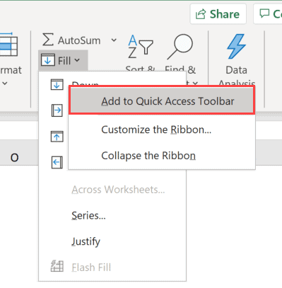
T0 add it to the Quick Access Toolbar (QAT), go to the ‘Fill Down’ option, right-click on it, and then click on ‘Add to the Quick Access Toolbar’
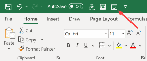
Now, you will see the ‘Fill Down’ icon appear in the QAT.
Using Keyboard Shortcut
If you prefer using the keyboard shortcuts, you can also use the below shortcut to achieve the fill down functionality:
CONTROL + D (hold the control key and then press the D key)
Below are the steps to use the keyboard shortcut to fill-down the formula:
- In cell A2, enter the formula: =B2*15%
- Select all the cells in which you want to apply the formula (including cell C2)
- Hold the Control key and then press the D key
Using Array Formula
If you’re using Microsoft 365 and have access to dynamic arrays, you can also use the array formula method to apply a formula to the entire column.
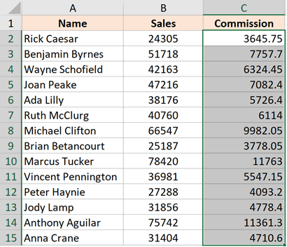
Suppose you have a data set as shown below and you want to calculate the Commission in column C.
Below is the formula that you can use:
=B2:B15*15%
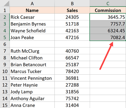
This is an Array formula that would return 14 values in the cell (one each for B2:B15). But since we have dynamic arrays, the result would not be restricted to the single-cell and would spill over to fill the entire column.
Note that you cannot use this formula in every scenario. In this case, because our formula uses the input value from an adjacent column and as the same length of the column in which we want the result (i.e., 14 cells), it works fine here.
But if this is not the case, this may not be the best way to copy a formula to the entire column
By Copy-Pasting the Cell
Another quick and well-known method of applying a formula to the entire column (or selected cells in the entire column) is to simply copy the cell that has the formula and paste it over those cells in the column where you need that formula.
Below are the steps to do this:
- In cell A2, enter the formula: =B2*15%
- Copy the cell (use the keyboard shortcut Control + C in Windows or Command + C in Mac)
- Select all the cells where you want to apply the same formula (excluding cell C2)
- Paste the copied cell (Control + V in Windows and Command + V in Mac)
One difference between this copy-paste method and all the methods convert below above this is that with this method you can choose to only paste the formula (and not paste any of the formattings).
For example, if cell C2 has a blue cell color in it, all the methods covered so far (except the array formula method) would not only copy and paste the formula to the entire column but also paste the formatting (such as the cell color, font size, bold/italics)
If you want to only apply the formula and not the formatting, use the steps below:
- In cell A2, enter the formula: =B2*15%
- Copy the cell (use the keyboard shortcut Control + C in Windows or Command + C in Mac)
- Select all the cells where you want to apply the same formula
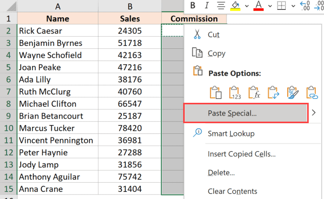
- Right-click on the Selection
- In the options that appear, click on ‘Paste Special’

- In the ‘Paste Special’ dialog box, click on the Formulas option

- Click OK
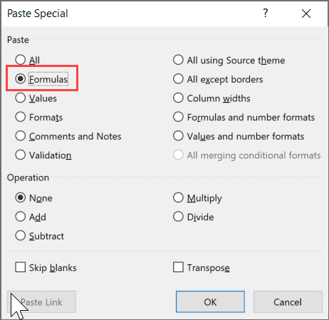
The above steps would make sure that only the formula is copied to the selected cells (and none of the formattings comes over with it).
So these are some of the quick and easy methods that you can use to apply a formula to the entire column in Excel.
I hope you found this tutorial useful!
Other Excel tutorials you may also like:
- 5 Ways to Insert New Columns in Excel (including Shortcut & VBA)
- How to Sum a Column in Excel
- How to Compare Two Columns in Excel (for matches & differences)
- Lookup and Return Values in an Entire Row/Column in Excel
- How to Copy and Paste Columns in Excel?
- Apply Conditional Formatting Based on Another Column in Excel
- How to Multiply a Column by a Number in Excel
Simple question:
I want to create a formula which, in column Cn, will compute the values of An * Bn.
example
column C1 = column A1 * column B1
column C2 = column A2 * column B2
column C3 = column A3 * column B3
…etc
all the way down to
column Cn = column An * column Bn
Thanks
asked Apr 9, 2010 at 5:31
![]()
Easy way to do it.
- Highlight your formula cell.
- The lower right corner should turn into a + sign.
- Click on that + sign and drag it for as many rows as you like.
Alternatively, you can do this:
- Highlight the formula cell.
- Ctrl+C to copy.
- Click on the C column.
- Hit enter.
Now with the second method, it may start to lock up on you because of the large number of cells it has to compute. Just hit escape and it’ll go back to normal (but some cells may not be filled in, depending on how early you hit escape.)
answered Apr 9, 2010 at 5:42
![]()
JoshJosh
3,2157 gold badges30 silver badges44 bronze badges
In what context are you trying to create a formula? If in VBA, you can do something like:
Range("A1").FormulaR1C1 = "=RC[-2]*RC[-1]"
This formula is in R1C1 format. It tells the system to take the value two columns to the left of the cell containing the formula and multiply it by the column to immediately to the left of the cell containing the formula. This same formula could be entered in all rows of column C and would automatically adjust based on the row.
answered Apr 9, 2010 at 5:41
![]()
ThomasThomas
63.5k12 gold badges94 silver badges140 bronze badges
Applying a formula is the most common task, but when we need to apply the same formula in the cells of an entire column, it becomes a tedious task. There are multiple ways to learn how to insert a formula for the entire column.
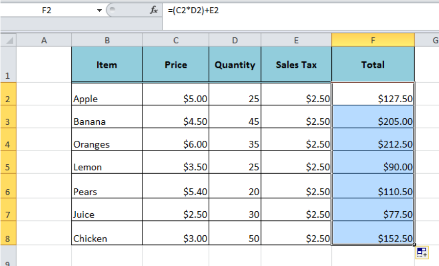 Figure 1. Applying Formula to an Entire Column
Suppose we have a list of items with given price, quantity and sales tax amount and we want to calculate the total amount for each item in column F by using the formula syntax
=(Price * Quantity) + Sales Tax
In cell F2, we apply the formula =(C2*D2)+E2 to calculate Total Amount. There are multiple ways to learn how to apply a formula to an entire column.
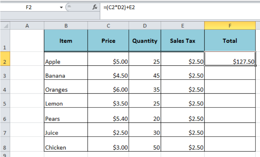 Figure 2. Excel Column Functions
By Dragging the Fill Handle
Once we have entered the formula in row 2 of column F, then we can apply this formula to the entire column F by dragging the Fill handle. Just select the cell F2, place the cursor on the bottom right corner, hold and drag the Fill handle to apply the formula to the entire column in all adjacent cells.
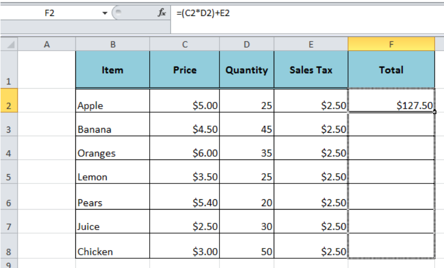 Figure 3. Dragging Fill Handle
By Double-Clicking Fill Handle
The easiest way to apply a formula to the entire column in all adjacent cells is by double-clicking the fill handle by selecting the formula cell. In this example, we need to select the cell F2 and double click on the bottom right corner. Excel applies the same formula to all the adjacent cells in the entire column F.
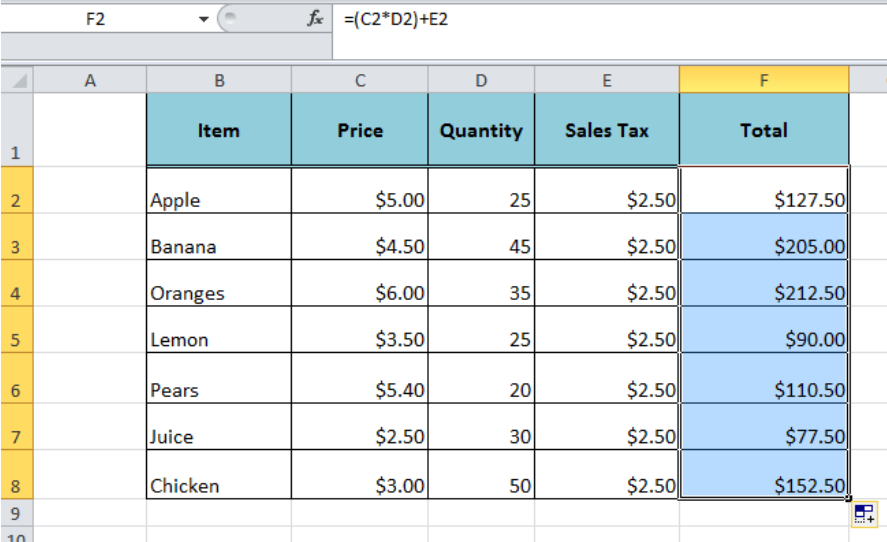 Figure 4. Double Click the Fill Handle
By Using Fill Command
Using Fill command is another good method to apply the formula to an entire column. We need to do the following to achieve for the entire column;
- After entering the formula in cell F2,
- Press Ctrl+Shift+End short keys. This will select the last used cell in the entire column.
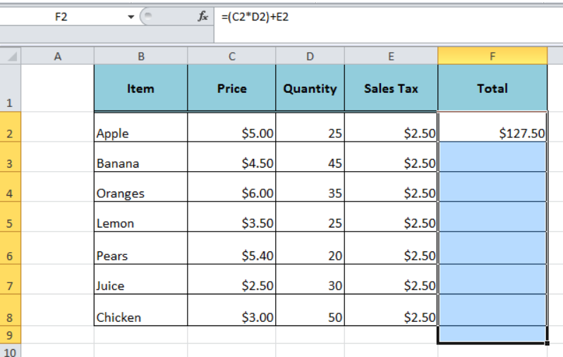 Figure 5. Selecting Last Used Cell in the Entire Column
- Go to Editing Group on Home tab, click in Fill arrow and select DOWN or alternately press Ctrl+D.
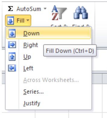 Figure 6. Using Fill Command
- Fill command applies the formula to all the selected cells.
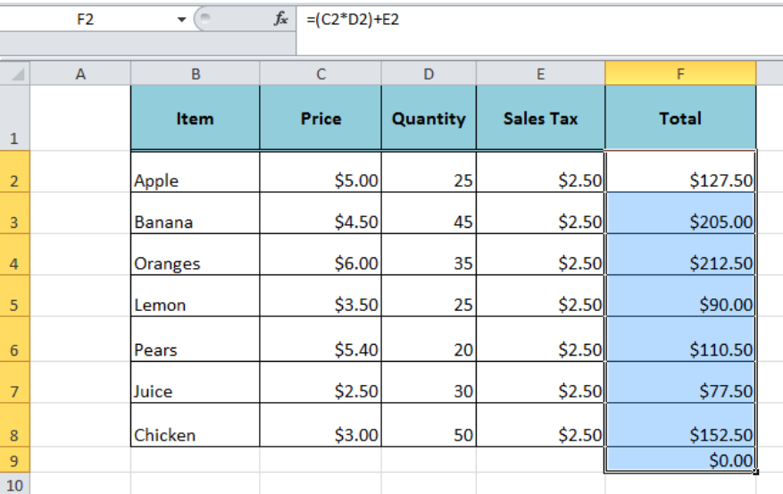 Figure 7. Column Function
Instant Connection to an Expert through our Excelchat Service
Most of the time, the problem you will need to solve will be more complex than a simple application of a formula or function. If you want to save hours of research and frustration, try our live Excelchat service! Our Excel Experts are available 24/7 to answer any Excel question you may have. We guarantee a connection within 30 seconds and a customized solution within 20 minutes.
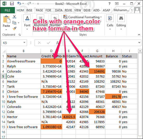
This tutorial talks about how to select cells with formula in Excel. In tutorial below I have compiled various methods to do the same. And the best part is that most the methods can select cells with formula without using any other third party software. I have also added a plugin in the following list to select cells in Excel that contain specific formula.
Selecting cells that contain formula or specific formula can be useful in many cases. Let’s say, you have an Excel sheet that has tons of cells in it with various formulas and you want to delete or change those cells. Doing it manually will take a fair amount of time. That’s where this tutorial comes in handy. In this tutorial I will explain how to select cells with formula in Excel.
You may already know how to select and count cells by background or font color. In the same way you can also select cells with formula in Excel with the help of the following methods. Let’s see how.
Do note that there could be various scenarios of selecting cells with formaula in Excel. You might want to simply select all the cells that have any formula, or you might want to select only those cells that have a spefic formula. I have explained all these scenarios here. If you have a selection scenario that I missed to cover here, do let me know in comments, and I will try to find a way for that as well.
This is the most basic scenario in which you want to simply select all the cells in a worksheet or selection that contain a formula. I will use the “Go to Special” tool of Excel to do the same. This Excel tool lets you select all the cells that have formula in them. Also, using the same tool, you can also select cells based on what is the output of formula in them. For example, you can choose to select only those cells in which formula would always product a numeric output (like, Sum, Avg, etc.).
To select cells that contain a formula, follow these simple steps.
Step 1: Open your Excel sheet in which you want to select the cells that have formula. And invoke Go to Special Tool from the Home ribbon.
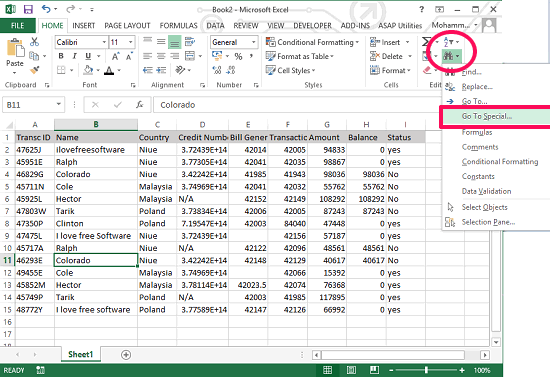
Step 2: From the Go To Special tool’s interface, check the Formula option and you can also filter the result by specifying the output type of the formula.
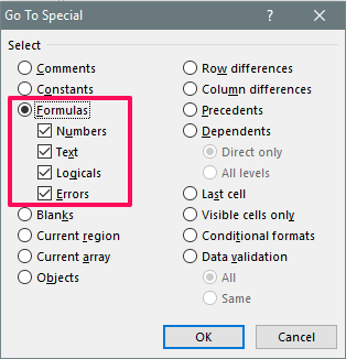
Step 3: To select all the cells containing a formula, hit the OK button. After that you will see all the cells that have formula have been selected.
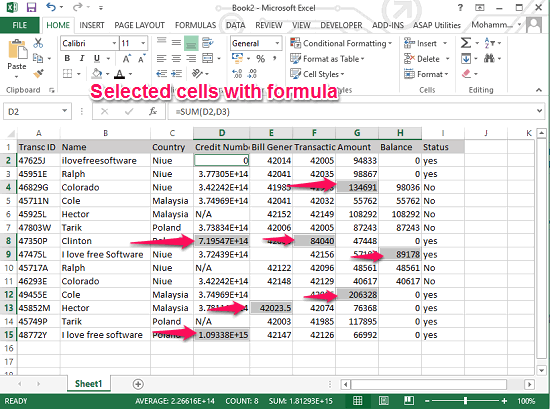
This is the fastest and easiest way to select cells with formula in Excel. And after you have your selected cells, you can do whatever you want to do with them.
How to Select Cells That Have a Specific Formula in Excel
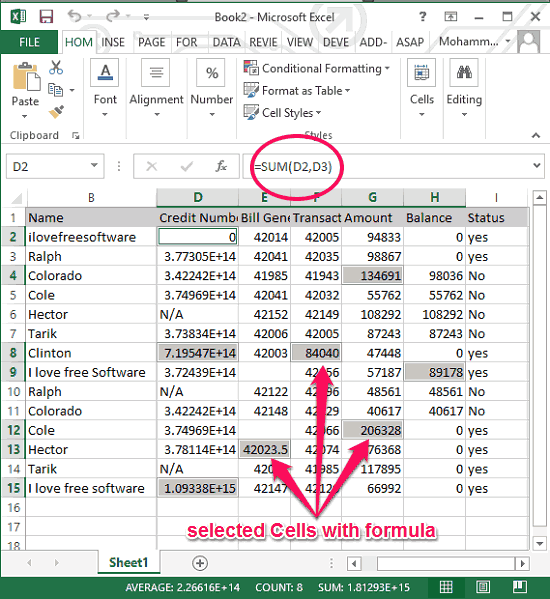
Let’s say you don’t want to select all the cells that have a formula, but only want to select those cells that have a specific formula. That is possible as well. You would be surprised to know that “Find” tool of the Excel will do it for you. The Find tool of Excel is very powerful. This tool can not only find the value, but also list all the cells that contain the specified formula text. And after that you can do whatever you want with the selected cells.
Follow these simple steps to select cells in Excel that contain a specific formula:
Step 1: Open any Excel sheet that contains cells with formula that you want to select. And click on the Find tool from the end of the Home tab of Excel. Or just to Ctrl+F.
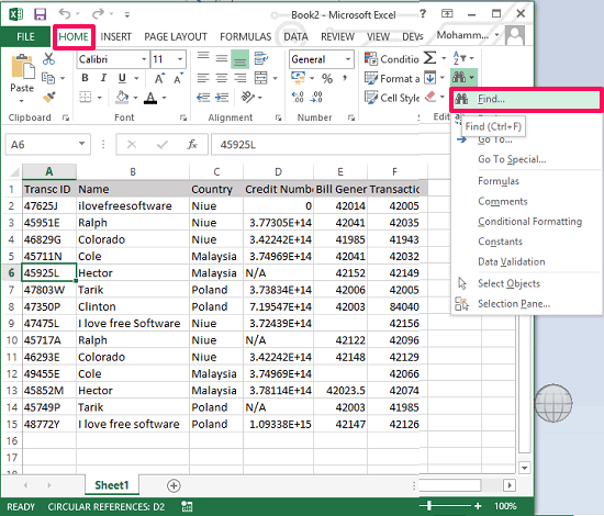
Step 2: Now, Expand the interface of the Find tool by clicking on the Options button. After that, navigate to “Look in” drop down and select “Formulas” from it.
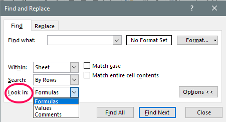
Step 3: Type the formula text in the “Find What” text box, and hit Find All button. You will see that it will list all the cells that contain that formula text.
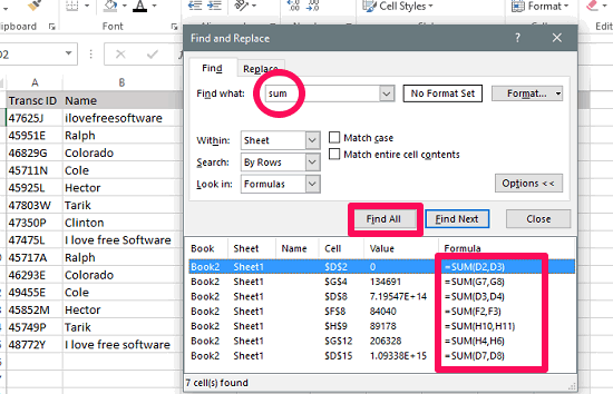
Now, if you want to select all the cells, click on any empty space in the result cells list and press Ctrl+A keyboard shortcut. After that, all the cells will get selected and you may now close the Find tool.
So, in this way you can easily select cells in Excel that contain a specific formula.
How to Select Cells With Formula in Excel that have a Specific font or font color
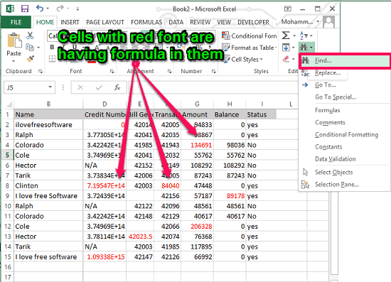
Let’s say you have a crazy scenario that you want to select all the cells in Excel that have a formula, and also they have a specific font, or a specific font color. I am not sure why you would run in this type of scenario, but in case you do, worry not. Here I have provided a solution for that too.
In this method I will use some filters along with the Find tool of Excel. After searching a specific formula text, the method will list all the cells that have the specified font or font color.
Here is how to do this:
Step 1: Open up any worksheet that contains some formatted cells and also have formulas in them. Open Find tool from the Home ribbon.
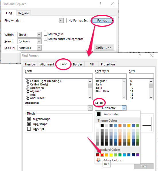
Step 2: Now, Expand the interface of the Find & Select tool by clicking on the Options button. After that, navigate to “Look in” drop down and select “Formulas” from it.
Step 3: Click on Format button and a window will pop up with various tabs it. Navigate to the Fonts tab and specify the font type there. For saving time, you can also directly specify font formatting from an existing cell from your sheet. To do this use the Choose Format From Cell button and specify the cell by selecting it from your Excel sheet.
Step 4: Type the formula text in the Find What text box, and hit Find All button. You will see that it will list all the cells that contain that formula text and has the font formatting that you selected.
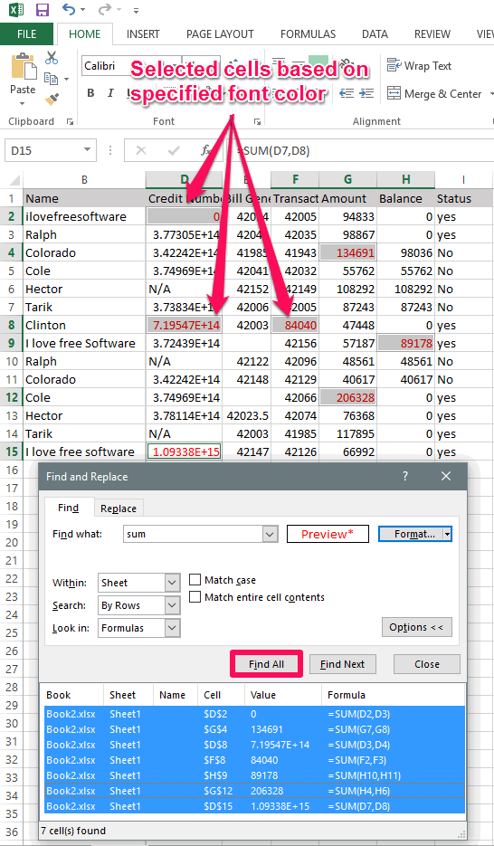
Now, if you want to select all the cells then click on any empty space in the result window and press the Ctrl+A keyboard shortcut. After that, all the cells will get selected and you may now close the Find & Select tool.
So, in this way you can select all the cells that contain a specific formula and font formatting. And you can do it in seconds.
Now, what if you want to select all the cells that had any formula, but have a specific formatting. For that, you can use Asap Utilities, that I have covered at the end of this tutorial.
Method 4: Select Cells With Formula in Excel That Have a Specific Background color
In the previous method I have explained how to select cells that contain specific formula and font. Now, in a similar way I will show how to select cells in Excel that have a specific formula and a specific background color. Let’s see how.
Step 1: Open an Excel sheet that has some colored cells with formulas in it. Invoke the Find tool using the keyboard shortcut Ctrl+F.
Step 2: After expanding the interface of the Find tool, configure it to search text in formulas as I have explained in above methods.
Step 3: Click on Format button and a window will pop up. Navigate to the Fill tab and specify the background color there. You can also directly specify the fill color from an existing cell of your sheet. To do this use the Choose Format From Cell button and specify the reference cell by selecting it from your Excel sheet.
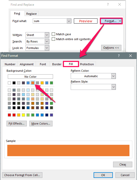
Step 4: Type the formula text in the Find What text box, and hit Find All button. You will see that it will list all the cells that contain that formula text and background color.
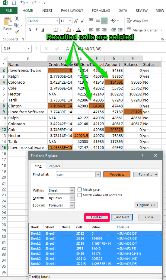
If you want to select all the cells, then click on any empty space in the result window and press the Ctrl+A keyboard shortcut. After that, all the cells will get selected and you can now close the Find tool.
So, in this way, you can select cells with formula in Excel and with the specified background color.
Bonus: Select Cells with Formula in Excel via Plugin
In the above mentioned methods I have explained how to select cells with formula in Excel and with the various formatting options. And for them I used built in functions of Excel. Now, in this section I will show you how you can do the same using an Excel plugin.
Asap Utilities package for Excel comes with tons of features to manipulate excel data that is difficult to do using the built in functions of Excel. However, it is only free for educational use.
One of the modules in the Asap Utilities package is Selecting cells based on content, formatting and more. I will use this tool of Asap Utilities to do the same. To see how to do it, simply follow these steps.
Step 1: Download and install Asap Utilities using this link. After installing it, you will see that it adds an additional tab in the Excel window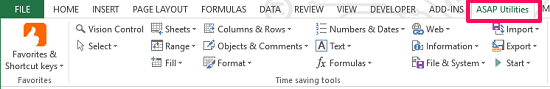
.Step 2: Open up any Excel sheet and navigate to the Asap Utilities tab and click on the Select drop down.
Step 3: Choose Selecting cells based on content, formatting and more option from the list and a window will pop up. And, you will have to configure various options there.
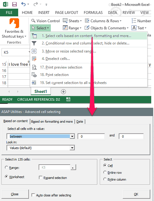
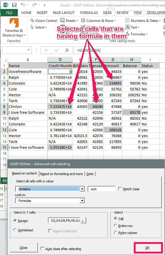
Step 4: Go to the first tab “Based on Content”. In this, choose “contains” from the first drop-down. And in the “Look in” drop down, choose “Formulas”.

Step 5: Type the name of the formula to be searched and hit the OK button.
At the end of the step 5, you will see that all the cells will get selected that meet with the specified condition.
So, it was the other nice way to select cells in Excel. If you are a plugin enthusiast, then you may give this method a try.
Also, if you want to select all cells that have a formula and have a specific formatting, then leave the drop-down next to “contains” blank. Then head over to “Based on formatting and more” and specify the formatting that you wish to select. In this way you will be able to select cells with formula and specific formatting.
Closing Thoughts
In the tutorial above, I have demonstrated various methods to select cells with formula in Excel. I have also explained to achieve the same with various criteria. So, if you are looking for the ways to do the same, then this tutorial should help you. Depending on what suits you need, you can give a try to any of the mentioned methods.