
Excel for Microsoft 365 Excel for Microsoft 365 for Mac Excel for the web Excel 2021 Excel 2021 for Mac Excel 2019 Excel 2019 for Mac Excel 2016 Excel 2016 for Mac Excel 2013 Excel 2010 Excel 2007 Excel for Mac 2011 Excel Starter 2010 More…Less
This article describes the formula syntax and usage of the FIND and FINDB functions in Microsoft Excel.
Description
FIND and FINDB locate one text string within a second text string, and return the number of the starting position of the first text string from the first character of the second text string.
Important:
-
These functions may not be available in all languages.
-
FIND is intended for use with languages that use the single-byte character set (SBCS), whereas FINDB is intended for use with languages that use the double-byte character set (DBCS). The default language setting on your computer affects the return value in the following way:
-
FIND always counts each character, whether single-byte or double-byte, as 1, no matter what the default language setting is.
-
FINDB counts each double-byte character as 2 when you have enabled the editing of a language that supports DBCS and then set it as the default language. Otherwise, FINDB counts each character as 1.
The languages that support DBCS include Japanese, Chinese (Simplified), Chinese (Traditional), and Korean.
Syntax
FIND(find_text, within_text, [start_num])
FINDB(find_text, within_text, [start_num])
The FIND and FINDB function syntax has the following arguments:
-
Find_text Required. The text you want to find.
-
Within_text Required. The text containing the text you want to find.
-
Start_num Optional. Specifies the character at which to start the search. The first character in within_text is character number 1. If you omit start_num, it is assumed to be 1.
Remarks
-
FIND and FINDB are case sensitive and don’t allow wildcard characters. If you don’t want to do a case sensitive search or use wildcard characters, you can use SEARCH and SEARCHB.
-
If find_text is «» (empty text), FIND matches the first character in the search string (that is, the character numbered start_num or 1).
-
Find_text cannot contain any wildcard characters.
-
If find_text does not appear in within_text, FIND and FINDB return the #VALUE! error value.
-
If start_num is not greater than zero, FIND and FINDB return the #VALUE! error value.
-
If start_num is greater than the length of within_text, FIND and FINDB return the #VALUE! error value.
-
Use start_num to skip a specified number of characters. Using FIND as an example, suppose you are working with the text string «AYF0093.YoungMensApparel». To find the number of the first «Y» in the descriptive part of the text string, set start_num equal to 8 so that the serial-number portion of the text is not searched. FIND begins with character 8, finds find_text at the next character, and returns the number 9. FIND always returns the number of characters from the start of within_text, counting the characters you skip if start_num is greater than 1.
Examples
Copy the example data in the following table, and paste it in cell A1 of a new Excel worksheet. For formulas to show results, select them, press F2, and then press Enter. If you need to, you can adjust the column widths to see all the data.
|
Data |
||
|
Miriam McGovern |
||
|
Formula |
Description |
Result |
|
=FIND(«M»,A2) |
Position of the first «M» in cell A2 |
1 |
|
=FIND(«m»,A2) |
Position of the first «M» in cell A2 |
6 |
|
=FIND(«M»,A2,3) |
Position of the first «M» in cell A2, starting with the third character |
8 |
Example 2
|
Data |
||
|
Ceramic Insulators #124-TD45-87 |
||
|
Copper Coils #12-671-6772 |
||
|
Variable Resistors #116010 |
||
|
Formula |
Description (Result) |
Result |
|
=MID(A2,1,FIND(» #»,A2,1)-1) |
Extracts text from position 1 to the position of «#» in cell A2 (Ceramic Insulators) |
Ceramic Insulators |
|
=MID(A3,1,FIND(» #»,A3,1)-1) |
Extracts text from position 1 to the position of «#» in cell A3 (Copper Coils) |
Copper Coils |
|
=MID(A4,1,FIND(» #»,A4,1)-1) |
Extracts text from position 1 to the position of «#» in cell A4 (Variable Resistors) |
Variable Resistors |
Need more help?
Функция НАЙТИ (FIND) в Excel используется для поиска текстового значения внутри строчки с текстом и указать порядковый номер буквы с которого начинается искомое слово в найденной строке.
Содержание
- Что возвращает функция
- Синтаксис
- Аргументы функции
- Дополнительная информация
- Примеры использования функции НАЙТИ в Excel
- Пример 1. Ищем слово в текстовой строке (с начала строки)
- Пример 2. Ищем слово в текстовой строке (с заданным порядковым номером старта поиска)
- Пример 3. Поиск текстового значения внутри текстовой строки с дублированным искомым значением
Что возвращает функция
Возвращает числовое значение, обозначающее стартовую позицию текстовой строчки внутри другой текстовой строчки.
Синтаксис
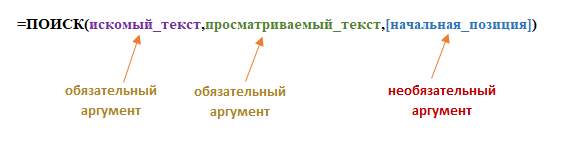
=FIND(find_text, within_text, [start_num]) — английская версия
=НАЙТИ(искомый_текст;просматриваемый_текст;[нач_позиция]) — русская версия
Аргументы функции
- find_text (искомый_текст) — текст или строка которую вы хотите найти в рамках другой строки;
- within_text (просматриваемый_текст) — текст, внутри которого вы хотите найти аргумент find_text (искомый_текст);
- [start_num] ([нач_позиция]) — число, отображающее позицию, с которой вы хотите начать поиск. Если аргумент не указать, то поиск начнется сначала.
Дополнительная информация
- Если стартовое число не указано, то функция начинает поиск искомого текста с начала строки;
- Функция НАЙТИ чувствительна к регистру. Если вы хотите сделать поиск без учета регистра, используйте функцию SEARCH в Excel;
- Функция не учитывает подстановочные знаки при поиске. Если вы хотите использовать подстановочные знаки для поиска, используйте функцию SEARCH в Excel;
- Функция каждый раз возвращает ошибку, когда не находит искомый текст в заданной строке.
Примеры использования функции НАЙТИ в Excel
Пример 1. Ищем слово в текстовой строке (с начала строки)

На примере выше мы ищем слово «Доброе» в словосочетании «Доброе Утро». По результатам поиска, функция выдает число «1», которое обозначает, что слово «Доброе» начинается с первой по очереди буквы в, заданной в качестве области поиска, текстовой строке.
Больше лайфхаков в нашем Telegram Подписаться
Обратите внимание, что так как функция НАЙТИ в Excel чувствительна к регистру, вы не сможете найти слово «доброе» в словосочетании «Доброе утро», так как оно написано с маленькой буквы. Для того, чтобы осуществить поиска без учета регистра следует пользоваться функцией SEARCH.
Пример 2. Ищем слово в текстовой строке (с заданным порядковым номером старта поиска)
Третий аргумент функции НАЙТИ указывает позицию, с которой функция начинает поиск искомого значения. На примере выше функция возвращает число «1» когда мы начинаем поиск слова «Доброе» в словосочетании «Доброе утро» с начала текстовой строки. Но если мы зададим аргумент функции start_num (нач_позиция) со значением «2», то функция выдаст ошибку, так как начиная поиск со второй буквы текстовой строки, она не может ничего найти.
Если вы не укажете номер позиции, с которой функции следует начинать поиск искомого аргумента, то Excel по умолчанию начнет поиск с самого начала текстовой строки.
Пример 3. Поиск текстового значения внутри текстовой строки с дублированным искомым значением
На примере выше мы ищем слово «Доброе» в словосочетании «Доброе Доброе утро». Когда мы начинаем поиск слова «Доброе» с начала текстовой строки, то функция выдает число «1», так как первое слово «Доброе» начинается с первой буквы в словосочетании «Доброе Доброе утро».
Но, если мы укажем в качестве аргумента start_num (нач_позиция) число «2» и попросим функцию начать поиск со второй буквы в заданной текстовой строке, то функция выдаст число «6», так как Excel находит искомое слово «Доброе» начиная со второй буквы словосочетания «Доброе Доброе утро» только на 6 позиции.
Purpose
Get location substring in a string
Return value
A number representing the location of substring
Usage notes
The FIND function returns the position (as a number) of one text string inside another. If there is more than one occurrence of the search string, FIND returns the position of the first occurrence. When the text is not found, FIND returns a #VALUE error. Also note, when find_text is empty, FIND returns 1. FIND does not support wildcards, and is always case-sensitive. Use the SEARCH function to find the position of text without case-sensitivity and with wildcard support.
Basic Example
The FIND function is designed to look inside a text string for a specific substring. When FIND locates the substring, it returns a position of the substring in the text as a number. If the substring is not found, FIND returns a #VALUE error. For example:
=FIND("p","apple") // returns 2
=FIND("z","apple") // returns #VALUE!
Note that text values entered directly into FIND must be enclosed in double-quotes («»).
Case-sensitive
The FIND function always case-sensitive:
=FIND("a","Apple") // returns #VALUE!
=FIND("A","Apple") // returns 1
TRUE or FALSE result
To force a TRUE or FALSE result, nest the FIND function inside the ISNUMBER function. ISNUMBER returns TRUE for numeric values and FALSE for anything else. If FIND locates the substring, it returns the position as a number, and ISNUMBER returns TRUE:
=ISNUMBER(FIND("p","apple")) // returns TRUE
=ISNUMBER(FIND("z","apple")) // returns FALSE
If FIND doesn’t locate the substring, it returns an error, and ISNUMBER returns FALSE.
Start number
The FIND function has an optional argument called start_num, that controls where FIND should begin looking for a substring. To find the first match of «the» in any combination of upper or lowercase, you can omit start_num, which defaults to 1:
=FIND("x","20 x 30 x 50") // returns 4To start searching at character 5, enter 4 for start_num:
=FIND("x","20 x 30 x 50",5) // returns 9
Wildcards
The FIND function does not support wildcards. See the SEARCH function.
If cell contains
To return a custom result with the SEARCH function, use the IF function like this:
=IF(ISNUMBER(FIND(substring,A1)), "Yes", "No")
Instead of returning TRUE or FALSE, the formula above will return «Yes» if substring is found and «No» if not.
Notes
- The FIND function returns the location of the first find_text in within_text.
- The location is returned as the number of characters from the start.
- Start_num is optional and defaults to 1.
- FIND returns 1 when find_text is empty.
- FIND returns #VALUE if find_text is not found.
- FIND is case-sensitive but does not support wildcards.
- Use the SEARCH function to find a substring with wildcards.
Функция ПОИСК осуществляет поиск текста, символа, цифры в указанной области. Она похожа на функцию НАЙТИ, которая так же ищет значение в указанной области, но у них есть отличия, которые мы разберем на примерах.
Как работает функция ПОИСК в Excel
Синтаксис данной функции выглядит следующим образом:
У нас есть слово «Excel». В этом примере нужно найти положение буквы «Х» в слове. Функция возвратит значение 2, поскольку буква находится по счету на втором месте в искомых данных:
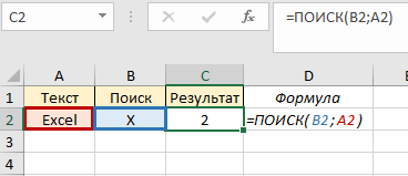
Несмотря на то, что искомая буква «Х» находится в верхнем регистре, функция нашла ее аналог в нижнем регистре и выдала результат. В этом и есть отличие с функцией НАЙТИ – она обращает внимание на соответствие регистров.
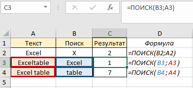
Также мы можем искать часть слова или слово в искомой области, например найти слово «Excel» в «Exceltable» и «table» во фразе «Excel table». В первом случае в результате мы получим 1, потому что слово «Excel» начинается с первого символа. Во втором случае у нас будет результат 7, потому что «table» начинается с седьмого символа:
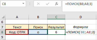
Аргумент начальная_позиция используем, когда нужно отсчитать положение символа, начиная с которого возвратится искомое значение. Например, нужно отследить с какой позиции начинается буквенное значение кода. Если не указать номер позиции, у нас возвратится число «2», поскольку буква «о» в ячейке А8 находится второй по порядку:
Благодаря этой функции можно возвращать части фраз, которые требует условие, а не только порядочное положение символа. Для этого функцию ПОИСК нужно комбинировать с другими функциями. Однако, такие комбинации функции могут быть довольно объёмными и существуют функции, более подходящие для выполнения таких задач.
Функция ПОИСКа значения в столбце Excel
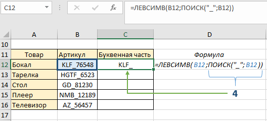
В данном примере будет использоваться формула комбинации функции ПОИСК с функциями: ЛЕВСИМВ, ПРАВСИМВ, ДЛСТР. Рассмотрим поэтапно пример, где мы сможем извлекать части фраз с текста, из которого получим искомое значение. У нас есть товар и артикул товара. Наше задание – возвратить только буквенную часть названия артикула. Для этого в ячейке C12 начинаем писать формулу. Для получения результата нам нужна функция ЛЕВСИМВ.
- Первый аргумент — текст, в котором происходит поиск (ячейка B12).
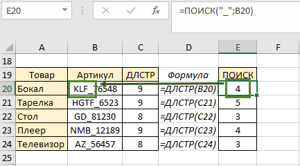
- Второй аргумент — нужна длина искомого слова. В первом артикуле она равна 3, а в последующих меняется, поэтому используем формулу ПОИСК(«_»;B12).
Формула с аргументами («_»;B12) указала, что будут возвращаться те символы, которые расположены перед символом нижнего подчеркивания. Проверим наш результат:
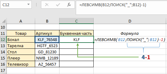
Функция ПОИСК возвратила число 4 (порядочное положение знака нижнего подчеркивания), и в качестве второго аргумента функции ЛЕВСИМВ указала какие символы будут находиться в ячейке С12. Пока что это не совсем то, что необходимо получить – знак «_» в идеале должен отсутствовать. Для этого немного подкорректируем формулу: перед вторым аргументом (формулой ПОИСК) отнимаем единицу, этим мы указали что вывод символов будет без знака нижнего подчеркивания (4-1):
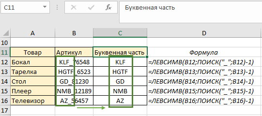
Поскольку формула у нас динамическая, копируем ее до конца столбца и наблюдаем результат нашей работы – по каждому артикулу мы получили буквенное значение независимо от количества букв:
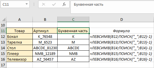
Если вдруг вам понадобится в этой же таблице изменить артикул – функция среагирует на изменения корректно и автоматически возвратит текстовое значение заменённого артикула. Например для товара «Бокал» будет буквенная часть «К», для «Тарелки» — «М», для «Стола» — ADCDE:
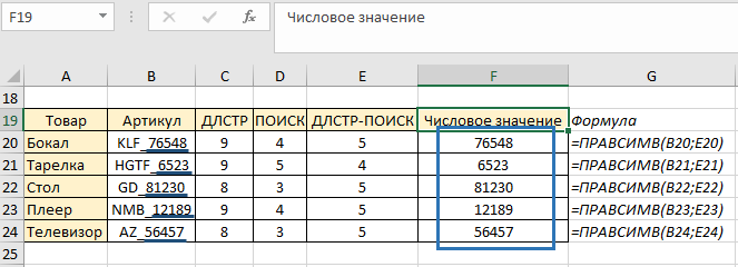
Теперь рассмотрим пример, где будем извлекать символы не ПЕРЕД нижним подчеркиванием, а ПОСЛЕ. В этом нам поможет функция ДЛСТР. Она помогает узнать длину текстовой строки. В ячейке С20 пишем формулу:
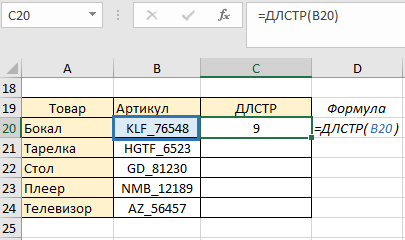
В результате она возвратила нам длину артикула товара «Бокал». Скопируем формулу до конца столбца и в следующем этапе в ячейке Е20 напишем формулу ПОИСК. Нижнее подчеркивание – это искомое значение (аргумент 1), возвращаемое значение – позиция порядковый номер положения нижнего подчеркивания. Копируем до конца столбца:
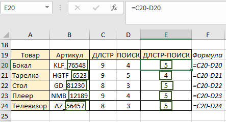
Затем нам нужен столбец, где мы от длины строки отнимаем позицию нижнего подчеркивания (9 — 4) и копируем формулу до конца столбца. То есть этот столбец содержит длину числового значения артикула (значения ПОСЛЕ нижнего подчеркивания):
Теперь в ячейке F20 пишем функцию ПРАВСИМВ, которая возвратит нам текст, часть фразы, которую мы запрашимаем. Первый аргумент функции – это ячейка, которую проверяет формула, а второй – длина возвращаемого значения:
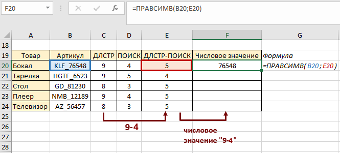
Функция возвратила нам числовое значение артикула товара. Копируем до конца столбца и получаем результат по каждому товару:
Данный пример был рассмотрен поэтапно для более понятного алгоритма выполнения задачи, однако можно числовое значение получить одним шагом:
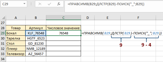
В этом примере мы сделали то же самое, что и ранее, только все операции сделали в одной формуле: нашли длину текста, отняли длину текста после знака «_» и возвратили эту длину функцией ПРАВСИМВ.
Как использовать функцию ПОИСК с функцией ЕСЛИ
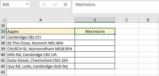
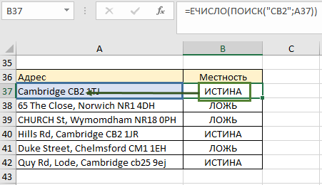
Рассмотрим пример, где будем проверять частичное совпадение текста в проверяемом тексте. У нас есть несколько адресов и нам нужно знать локальные они или нет:
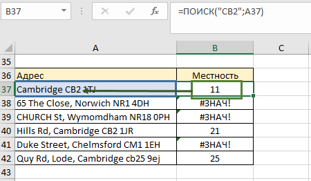
Если почтовый индекс начинается с СВ2, тогда это локальный адрес. Мы не можем использовать функцию ЕСЛИ в её обычном выражении, потому что в ячейках много другого текста. Нам нужно знать содержит ли ячейка часть «СВ2». Чтобы лучше понимать логику построения функции, будем делать это от простого к более сложному выражению:
- Строим функцию ПОИСК: 1-й аргумент – «СВ2», 2-й аргумент – ячейка А37, копируем до конца столбца. Так мы указали что и где будем искать. Там, где нет текста СВ2, возвратилась ошибка. Но сейчас у нас есть только номер позиции текста СВ2. А функция ЕСЛИ будет искать идентичное совпадение. То есть она будет искать число 11 в тексте ячейки А37, которого у нас, конечно, не будет нигде.
- Формулу функции ПОИСК вкладываем в функцию ЕЧИСЛО (имеет только 1 аргумент), которая будет указателем в дальнейшем для ЕСЛИ, что результатом функции ПОИСК является число (как сейчас, у нас 11):
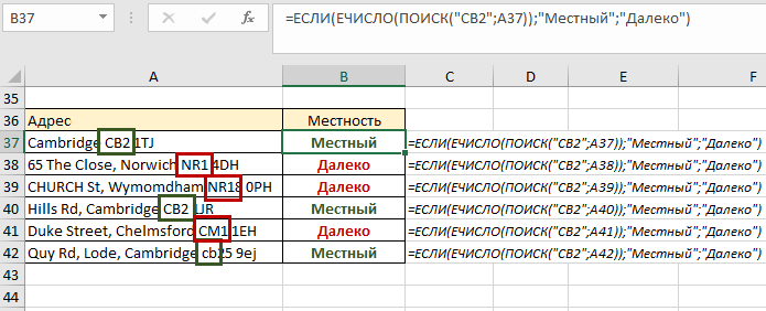
- Полученную формулу вкладываем в ЕСЛИ, указывая, что для значения ИСТИНА у нас будет слово «Местный», а для значения ЛОЖЬ – «Далеко». Копируем до конца столбца:
 Скачать примеры формул с функцией ПОИСК в Excel
Теперь у нас есть информация об адресах в зависимости от их почтового индекса. Вполне логичное предположение, что можно также было использовать НАЙТИ, но поскольку НАЙТИ учитывает регистр, полезнее и надежнее будет работа с ПОИСКом.
Find in Excel (Table of Contents)
- Using Find and Select Feature in Excel
- FIND Function in Excel
- SEARCH Function in Excel
Introduction to Find in Excel
There are two ways to find it in Excel. First, we can use Find by pressing Ctrl + F shortcut keys. Therein Find and Replace box, search the word or field which we want to find in the Find What section. In another way, we can use the FIND function. For this, select the Find function from the insert function and, as per syntax, select the substring from where we need to find it, and choose the word or letter or number which we want to find in the String position. This will return the position of the chosen string from the selected Substring.
Methods to Find in Excel
Below are the different methods to find in excel.
You can download this Find in Excel Template here – Find in Excel Template
Method #1 – Using Find and Select Feature in Excel
Let’s see How to Find a Number or a Character in Excel using the Find and Select feature in Excel.
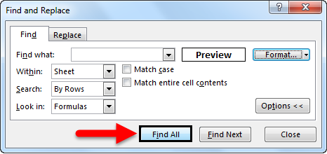
Step 1 – Under the Home tab, in the Editing group, click Find & Select.
Step 2 – To find text or numbers, click Find.
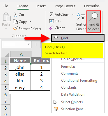
- In the Find what box, type the text or character you want to search for, or click the arrow in the Find what box and then click a recent search in the list.
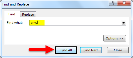
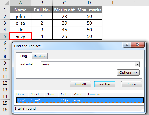
Here, we have a record of marks of four students. Suppose we want to find the text ‘envy’ in this table. For this, we click Find and Select under the Home tab then the Find and Replace dialog box appears. In the Find what box, we enter ‘envy’ then click on Find All. We get the text ‘envy’ is in cell number A5.
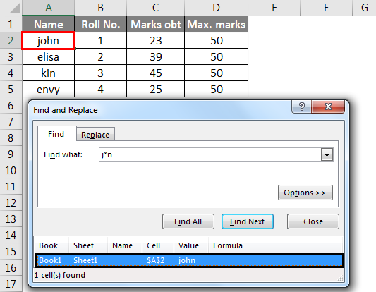
- You can use wildcard characters, such as an asterisk (*) or a question mark (?), in your search criteria:
Use the asterisk to find any string of characters.
Suppose we want to find text in the table which starts with the letter ‘j’ and ends with the letter ‘n’. In the Find and Replace dialog box, we enter ‘j*n’ in the Find what box, then click on Find All.
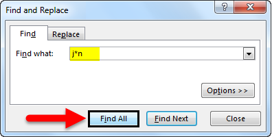
We will get the result as text ‘j*n’(john) is in the cell no. ‘A2’ because we have only one text which starts with ‘j’ and ends with ‘n’ with any number of characters between them.
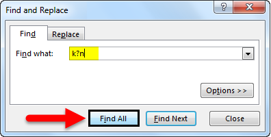
Use the question mark to find any single character.
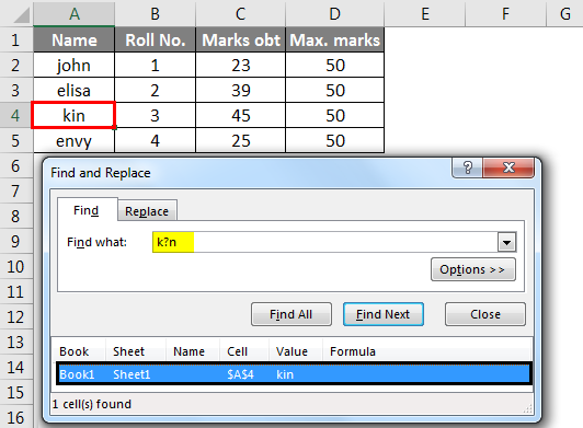
Suppose we want to find text in the table that starts with the letter ‘k’ and ends with the letter ‘n’ with a single character. So, in the Find and Replace dialog box, we enter ‘k?n’ to find what box. Then click on Find All.
Here, we get the text ‘k?n’(kin) is in cell no. ‘A4’ because we have only one text which starts with ‘k’ and ends with ‘n’ with a single character between them.
- Click Options to further define your search if needed.
- We can find text or number by changing settings in the Within, Search and Look in the box according to our needs.
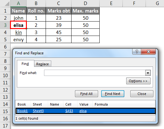
- To show the working of the above-mentioned options, we took the data as follows.
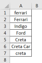
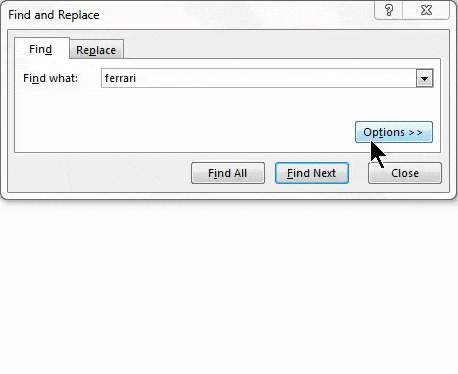
- To search case-sensitive data, select the Match case check box. It gives you output in the case you give input in the Find What box. For example, we have a table of some cars’ names. If you type ‘ferrari’ in the Find What box, then it will find only ‘ferrari’, not ‘Ferrari’.
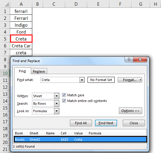
- To search for cells that contain just the characters you typed in the Find what box, select the Match entire cell contents checkbox. For example, we have a table of some cars’ names. Type ‘Creta’ in the Find What box.
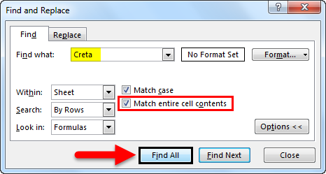
- It will then find cells containing exactly ‘Creta’, and cells containing ‘Cretaa’ or ‘Creta car’ will not be found.
- If you want to search for text or numbers with specific formatting, click Format, and then make your selections in the Find Format dialog box according to your need.
- Let us click the Font option and select the Bold, and click OK.
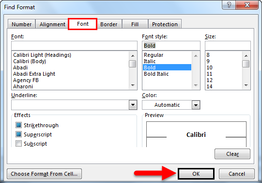
- Then, we click on Find All.
We get the value as ‘elisa’, which is in the ‘A3’ cell.
Method #2 – Using FIND Function in Excel
The FIND function in Excel gives the location of a substring within a string.
Syntax For FIND in Excel:
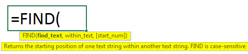
The first two parameters are required, and the last parameter is non-compulsory.
- Find_Value: The substring which you want to find.
- Within_String: The string in which you want to find the specific substring.
- Start_Position: It is a non-compulsory parameter and describes from which position we want to search substring. If you do not describe it, then start the search from the 1st position.
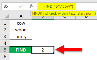
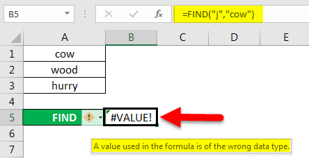
For example =FIND(“o”, “Cow”) gives 2 because “o” is the 2nd letter in the word “cow“.
FIND(“j”, “Cow”) gives an error because there is no “j” in “Cow”.
- If the Find_Value parameter contains multiple characters, the FIND function gives the location of the first character.
E.g., the formula FIND(“ur”, “hurry”) gives 2 because “u” in the 2nd letter in the word “hurry”.

- If Within_String contains multiple occurrences of Find_Value, the first occurrence is returned. For example, FIND (“o”, “wood”)
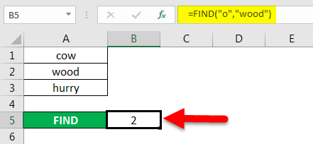
gives 2, which is the location of the first “o” character in the string “wood”.
The Excel FIND function gives the #VALUE! error if:
- If Find_Value does not exist in Within_String.
- If Start_Position contains multiple characters as compared to Within_String.
- If Start_Position either has a zero or negative number.
Method #3 – Using SEARCH Function in Excel
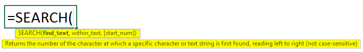
The SEARCH function in Excel is simultaneous to FIND because it also gives the location of a substring in a string.
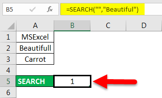
- If Find_Value is the blank string “, the Excel FIND formula gives the string’s first character.
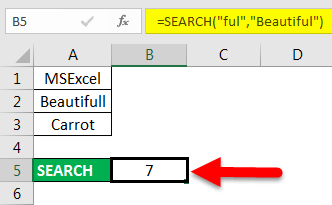
Example =SEARCH (“ful“, “Beautiful) gives 7 because the substring “ful” begins at the 7th position of the substring “beautiful”.
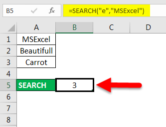
=SEARCH (“e”, “MSExcel”) gives 3 because “e” is the 3rd character in the word “MSExcel” and ignoring the case.
- Excel’s SEARCH function gives the #VALUE! error if:
- If the value of the Find_Value parameter is not found.
- If the Start_Position parameter is superior to the length of Within_String.
- If the Start_Position either equal to or less than 0.
Things to Remember About Find in Excel
- Asterisk defines a string of characters, and the question mark defines a single character. You can also find asterisks, question marks, and tilde characters (~) in worksheet data by preceding them with a tilde character inside the Find what option.
For example, to find data that contain “*”, you would type ~* as your search criteria.
- If you want to find cells that match a specific format, you can delete any criteria in the Find what box and select a specific cell format as an example. Click the arrow next to Format, click Choose Format From Cell, and click the cell with the formatting you want to search for.
- MSExcel saves the formatting options you define; you should clear the formatting options from the last search by clicking on an arrow next to Format and then Clear Find Format.
- The FIND function is case sensitive and does not allow while using wildcard characters.
- The SEARCH function is case-insensitive and allows while using wildcard characters.
Recommended Articles
This is a guide to Find in Excel. Here we discuss how to use the Find feature, Formula for FIND, and SEARCH in Excel, along with practical examples and a downloadable excel template. You can also go through our other suggested articles –
- FIND Function in Excel
- Excel SEARCH Function
- Find and Replace in Excel
- Search For Text in Excel