Формула факториала для excel

Excel для Microsoft 365 Excel для Microsoft 365 для Mac Excel для Интернета Excel 2021 Excel 2021 для Mac Excel 2019 Excel 2019 для Mac Excel 2016 Excel 2016 для Mac Excel 2013 Excel 2010 Excel 2007 Excel для Mac 2011 Excel Starter 2010 Еще…Меньше

Предположим, что у вас шесть колокольчиков с разными тонами и вы хотите найти количество уникальных последовательностей, в которых каждый колокольчик можно запускать один раз. В этом примере вычисляются факториал из шести. Как правило, с помощью факториала можно подсчитать количество способов у организовать группу отдельных элементов (также называемых перестроениями). Чтобы вычислить факториал числа, используйте функцию ФАКТЫ.

В этой статье описаны синтаксис формулы и использование функции ФАКТР в Microsoft Excel.

Описание

Возвращает факториал числа. Факториал числа — это значение, равное 1*2*3*…* число.

Синтаксис

ФАКТР(число)

Аргументы функции ФАКТР описаны ниже.

  • Число    — обязательный аргумент. Неотрицательное число, для которого вычисляется факториал. Если число не является целым, оно усекается.

Пример

Скопируйте образец данных из следующей таблицы и вставьте их в ячейку A1 нового листа Excel. Чтобы отобразить результаты формул, выделите их и нажмите клавишу F2, а затем — клавишу ВВОД. При необходимости измените ширину столбцов, чтобы видеть все данные.

Формула

Описание

Результат

=ФАКТР(5)

Факториал числа 5 или 1*2*3*4*5

120

=ФАКТР(1,9)

Факториал целой части числа 1,9

1

=ФАКТР(0)

Факториал числа 0

1

=ФАКТР(-1)

Факториал отрицательного числа возвращает значение ошибки

#ЧИСЛО!

=ФАКТР(1)

Факториал числа 1

1

Нужна дополнительная помощь?

Факториал в Excel

В этой статье я расскажу о факториале, его свойствах и о том, как вычислить его значение с помощью Excel. Мы проверим, как точно вычисляет значение факториала формула Стирлинга и разберем решение типовых задач с факториалами, а на закуску — несколько видеороликов (и конечно расчетный файл эксель). Удачи!

Полезная страница? Сохрани или расскажи друзьям

Что такое факториал?

Символ $n!$ называется факториалом и обозначает произведение всех целых чисел от $1$ до $n$. Факториал определен только для целых неотрицательных чисел.

$$n!=1cdot 2cdot 3 cdot … cdot (n-1) cdot n$$

По определению, считают, что $0!=1, 1!=1$. Далее:

$$
2!=1 cdot 2 = 2,\
3!=1 cdot 2 cdot 3= 6,\
4!=1 cdot 2 cdot 3cdot 4= 24,\
5!=1 cdot 2 cdot 3cdot 4cdot 5= 120,\

$$

Факториал растет невероятно быстро (недаром он обозначается восклицательным знаком!), существенно быстрее степенной $x^n$ или даже экспоненциальной функции $e^n$ (но медленее чем $e^{e^n}$)

Факториал широко применяется в комбинаторике — он равен числу всех перестановок $n$-элементного множества, а также входит в формулы для числа сочетаний и размещений. Факториал встречается в математическом анализе (чаще при разложениях функции в степенные ряды), а также в функциональном анализе и теории чисел.

Еще: онлайн калькулятор факториала.

Формулы и свойства факториала

Рекуррентная формула для факториала:

$$
n!=left{
begin{matrix}
1, & n=0,\
(n-1)!cdot n, & n gt 0.\
end{matrix}
right.
$$

Факториал связан с гамма-функцией по формуле: $n!= Gamma(n+1)$. Фактически, гамма-функция — обобщение понятия факториала на все положительные вещственные функции.

Для любого натурального $n$ выполняется:

$$
(n!)^2 ge n^n ge n! ge n.
$$

Любопытная формула связывает факториал и производную степенной функции:

$$ (x^n)^{(n)} = n!$$

Формула Стирлинга

Для приближенного вычисления факториала применяют асимптотическую формулу Стирлинга:

$$
n!=sqrt{2pi n} left( frac{n}{e}right )^n left(1+ frac{1}{12n}+ frac{1}{288n^2}- frac{139}{51840n^3}- frac{571}{2488320n^4}+… right )
$$

Обычно для расчетов берут только главный член:

$$
n! approx sqrt{2pi n} left( frac{n}{e}right )^n.
$$

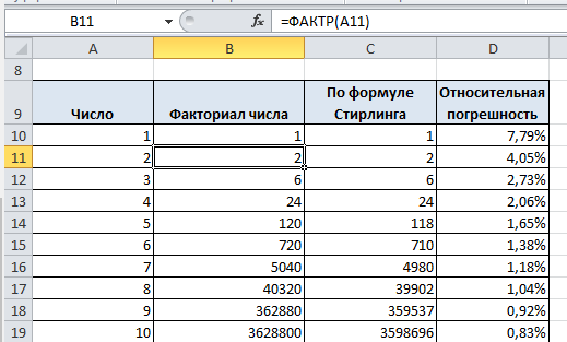
Ниже вы увидите пример расчета факториала по обычной формуле и с помощью формулы Стирлинга, которая, как видно, дает вполне хорошее приближение (начиная с $n=9$ относительная погрешность уже меньше 1%).

Расчет факториала в Эксель

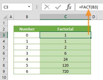
Для нахождения факториала в Excel нужно использовать специальную функцию =ФАКТР($n$), где $n$ — число, факториал которого нужно найти.

Пример расчета и ввода формулы ниже на скриншоте, также вы можете скачать расчетный файл

факториал в Excel

Нужна помощь в решении задач по комбинаторике?

Примеры задач с факториалом

Рассмотрим решение типовых задач.

Пример 1. На полке стоят 8 дисков. Сколькими способами их можно расставить между собой?

Решение. Требуется найти число всех перестановок 8 различных объектов, что вычисляется как раз как факториал:

$$N=8!=1 cdot 2 cdot 3cdot 4cdot 5cdot 6cdot 7cdot 8=40320.$$

Пример 2. Вычислить

$$
frac{60!}{58!}-frac{6!}{5!}
$$

Решение.

$$
frac{60!}{58!}-frac{6!}{5!}=frac{58!cdot 59cdot 60}{58!}-frac{5! cdot 6}{5!}=59cdot 60-6=3534.
$$

Пример 3. Упростить выражение

$$
frac{n+3}{(n+1)!}-frac{1}{n!}
$$

Решение.

$$
frac{n+3}{(n+1)!}-frac{1}{n!} = frac{n+3}{(n+1)!}-frac{n+1}{n!(n+1)}=frac{n+3-(n+1)}{(n+1)!}= frac{2}{(n+1)!}
$$

Пример 4. Упростить дробь, содержащую факториал:

$$
frac{n!}{(n-2)!}
$$

Решение.

$$
frac{n!}{(n-2)!}=frac{ (n-1)! cdot n}{(n-2)!} =frac{(n-2)! cdot (n-1) cdot n}{(n-2)!} = (n-1) cdot n = n^2-n$$

Видео о факториале

Небольшое учебное видео про факториал — определение, свойства, как быстро растет, как вычислить в Excel по встроенной формуле и по приближенной формуле Стирлинга.

Расчетный файл из видео можно скачать

Напоследок — насколько быстро растет факториал!

Полезные ссылки

  • Онлайн калькуляторы
  • Формулы комбинаторики в Excel
  • Примеры решений
  • Как решать задачи по комбинаторике?
  • Видеоуроки по комбинаторике
  • Решение на заказ

Решебник задач по комбинаторике

Понял, что на нашем сайте очень мало описаний математических функций. Хотя в Excel их превеликое множество. Есть описание НДС, всяких там печатных документов и форм. А вот описания основы основ табличного редактора — математических функций, почти нет. «Надо бы заняться этим пробелом» — подумал я. Вот занимаюсь. Первым на очереди факториал. Почему? Просто на днях делал одну задачу с этой функцией. Подробнее про факториал в Excel читаем далее.

Факториал в Excel. Введение

Думаю, углубляться в мат. часть сильно не стоит. Считаю, нужно рассказать, для чего используется эта функция и как ее считать в Excel.

Начнем с определения. Как говорит нам Википедия — Факториал числа n (от лат. factorialis — умножающий, действующий) — это произведение всех натуральных чисел от 1 до n включительно.

Для чего это может понадобиться? В первую очередь — это обозначение умножения нескольких чисел 3! = 1*2*3. Факториал очень часто используется в комбинаторике. Что такое комбинаторика? Как следует из названия — это наука изучающая математические комбинации.

Пример: Сколько сочетаний цветов получится из 10 разных цветов? Сходу знаете? Я, например, нет. Для вычисления кол-ва комбинаций применяется факториал.

Рассчитаем для 3 цветов: количество комбинаций цветов (желтый, красный, зеленый) = 3! =1*2*3 = 6. Какие это комбинации:

  1. ЖКЗ
  2. ЖЗК
  3. КЖЗ
  4. КЗЖ
  5. ЗЖК
  6. ЗКЖ

Действительно 6 :)

В более сложных задачах в жизни часто нужно узнать, к примеру, какое количество вариантов выполнения маршрута из 7 точек. Как видите, штука полезная!

Факториал в Excel. Как посчитать.

Для факториала есть специальная функция =ФАКТР() Реквизиты предельно просты: один аргумент, то число до которого нужно рассчитать факториал

Пример такой формулы

=ФАКТР(A1)

Факториал в Excel

Рассчитав факториал 7, мы узнаем, что количество вариантов маршрута из 7 точек равно 5040. По-моему, это впечатляет!

Удачной комбинаторики!

Вычисление факториала натуральных (неотрицательных целых) чисел с помощью пользовательской функции Factorial. Ограничение для VBA Excel по типу данных.

Факториал и его вычисление

Факториал – это функция, определяемая для натурального числа n как произведение всех неотрицательных целых чисел от 1 до n включительно.

Формула, по которой вычисляется факториал, записывается следующим образом:

n! = 1 · 2 · ... · n

Пример: 3! = 1 · 2 · 3 = 6

В соответствии с формулой факториала, будет верным следующее соотношение:

(n-1)! = n! : n

Если принять для этого равенства n = 1, тогда получим:

0! = 1

Пользовательская функция Factorial

Для вычисления факториала натуральных чисел можно использовать следующую пользовательскую функцию:

1

2

3

4

5

6

7

8

9

10

11

12

13

14

15

16

17

18

Public Function Factorial(n)

Dim i, p

    If Not IsNumeric(n) Or n = Empty Then

        Factorial = «Аргумент не является числом»

        Exit Function

    ElseIf n < 0 Then

        Factorial = «Аргумент отрицательный»

        Exit Function

    End If

p = 1

n = Format(n, 0)

    If n > 1 Then

        For i = 2 To n

            p = p * i

        Next

    End If

Factorial = p

End Function

Первое условие функции Factorial (If Not IsNumeric(n) Or n = Empty) проверяет, не является ли значение ячейки не числом. Второе условие (ElseIf n < 0) проверяет, не является ли число в ячейке отрицательным.

Если значение ячейки окажется не числом или числом отрицательным, функция возвратит соответствующее сообщение и завершит работу (Exit Function).

Далее, если функция Factorial не завершила работу, переменной p присваивается значение 1, которое возвратит функция, если значение переменной n будет равно нулю или единице.

Значение ячейки (переменная n) округляется до целого и, если оно окажется больше единицы, вычисляется факториал с помощью цикла For… Next.

Пользовательская функция Factorial возвратит значение, присвоенное ей из переменной p.

Рекурсивная функция Factorial

Рекурсивной называется функция, которая вызывает сама себя.

Рекурсивная функция, вычисляющая факториал:

Function Factorial(n)

    If n <= 1 Then

        Factorial = 1

    Else

        Factorial = Factorial(n 1) * n

    End If

End Function

Как она работает, я не понимаю, но она работает!

Ограничение по типу данных

Максимальное значение пользовательской функции Factorial для ячеек с общим форматированием будет ограничено максимальным значением типа данных Double (1,79769313486232Е+308).

Максимально возможное значение будет превышено при вычислении факториала при n > 170. В этом случае, в ячейку с функцией Factorial, Excel возвратит сообщение об ошибке: #ЗНАЧ!.

При желании, можно в код функции Factorial добавить еще одно условие, проверяющее, не содержит ли переменная n значение больше 170. Если n > 170, тогда вывод сообщения об этом и выход из функции.

Попробуйте задать ячейке с функцией Factorial числовой тип без дробных значений. У меня в Excel 2016 x64 факториал от 146 отображается из 15 значащих цифр впереди и огромного количества нулей справа. Чтобы это увидеть, надо ячейку растянуть на всю ширину и уменьшить размер шрифта в ней. Значение факториала от 147 в ячейке с числовым форматом уже не отображается.

Факториал числа часто используется, например, для расчета количества перестановок или вычисления биномиальных коэффициентов.
Рассмотрим особенности использования факториала в Excel.

Для начала освежим в памяти что же такое факториал числа.
Факториал числа n — произведение натуральных чисел от 1 до n (включительно), обозначается как n!.
В общем виде формула расчета факториала имеет вид n!=1*2*3*…*n, при этом по умолчанию считается, что 0!=1.
Наибольшее применение факториал имеет в комбинаторике и теории чисел.

Перейдем от теории к практике.
Для расчета факториала в Excel применяется функция ФАКТР:

ФАКТР(число)
Возвращает факториал числа, равный 1*2*3*…*число.

  • Число (обязательный аргумент) — натуральное число (т.е. целое неотрицательное), факториал которого вычисляется.

Функция факториала числа в Excel
В случае, если в качестве аргумента функции было введено нецелое число, то оно округляется в меньшую сторону.

Удачи вам и до скорой встречи на страницах блога Tutorexcel.ru!

Поделиться с друзьями:
Поиск по сайту:

What is a factorial?

A factorial calculates the ‘product’ of all numbers less than or equal to a value. For example, the factorial of 5 would be:

5x4x3x2x1=120

In mathematical notation, factorials are usually indicated with an exclamation mark. 5! would indicate the factorial of 5.

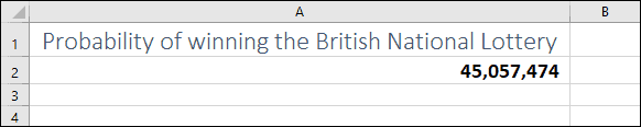
Factorials are typically used to calculate a number of possible combinations (or permutations). For example, the British National Lottery sells lottery tickets that contains 6 numbers from 1 to 59. The mathematical formula to calculate the total possible combinations of numbers is:

59!/(6!*(59-6)!)

This results in a value of 45,057,474, showing that a single ticket has a 1 in 45,057,474 chance of winning the British National Lottery!

Factorials in Excel

Because the exclamation mark is the symbol for a factorial you might expect it to be recognized by Excel, but you will get an error message if you try to enter a formula such as =5!.

To calculate factorials in excel you must use the FACT function.

=FACT(5) would calculate the factorial of 5 in Excel.

If you’re unfamiliar with Excel formulas and functions you could benefit greatly from our completely free Basic Skills E-book.

Many more advanced functions are explained in depth in our Expert Skills Books and E-books.

Calculating the probability of winning the lottery in Excel

Now that you know how to use the FACT function, it’s a simple matter to translate the mathematical formula shown above into an Excel formula:

=FACT(59)/(FACT(6)*FACT(59-6))

You can download an example workbook showing this in action.

Other combinatorial functions in Excel

Excel also contains a number of other useful ‘combinatorial’ functions. One of the most useful is COMBIN. COMBIN makes the calculation shown above even easier, as it allows you to return the total number of possible combinations from a given number of items. You can calculate the probability of winning the lottery with the simple formula:

=COMBIN(59,6)

Excel also offers the COMBINA function, which works the same way but allowing repetition of numbers. If you were allowed to choose the same number more than once in the lottery there would be 74,974,368 possible combinations and it would be much harder to win!

These are the only up-to-date Excel books currently published and includes the new Dynamic Arrays features.

They are also the only books that will teach you absolutely every Excel skill including Power Pivot, OLAP and DAX.

Some of the things you will learn

Share this article

Recent Articles

2 Responses

  1. I have tried 4! and the answer in excel is 24 (wrong) repeated many times. think you have a bug?

  2. Hi Pete

    The factorial of 4 is indeed 24:

    4*3*2*1 = 24

    … and if you use the formula =FACT(4) in Excel it will correctly return 24.

Leave a Reply

The Excel FACT function is a Math formula that returns the factorial of a given number. Factorial of a number n (denoted as n!) is the product of all numbers that are less than or equal to that number (n! = n x (n-1) x (n-2) x … x 2 x 1).  Frequently used in probability and statistics, Excel factorial calculations are fairly simple to execute. In this guide, we’re going to show you how to use the FACT function and also go over some tips and error handling methods.


Supported versions

  • All Excel versions

Excel FACT Function Syntax


Arguments

number

The number to be used in a factorial calculation. It must be greater than or equal to 0.


Examples

Common Use Cases

Let’s take a simple combination example. Say you have 3 dishes to serve 3 people, and want to find out in how many different ways you can serve the dishes. You need to find the permutation of the dishes by using the following formula.

Other Examples

You can’t calculate the factorial of a negative or a decimal number. While negative numbers will give a #NUM! error, decimal numbers will be truncated.

Download Workbook


Summary and Tips

  • If any of the values entered as an argument is not an integer, it will be truncated.
  • Use the FACTDOUBLE function to calculate the double factorial of a number.
  • The factorial of zero (0!) is equal to 1.

Issues

  • If any argument is a negative number, the FACT function returns a #NUM! error.
Date yes Add (Subtract) Days to a Date Concatenate Dates Convert Date to Number Convert Date to Text Month Name to Number Create Date Range from Dates Day Number of Year Month Name from Date First Day of Month Add (Subtract) Weeks to a Date If Functions with Dates Max Date Number of Days Between Dates Number of Days in a Month Number of Weeks Between Dates Number of Years Between Dates Split Date & Time into Separate Cells Countdown Remaining Days Insert Dates Random Date Generator Using Dynamic Ranges — Year to Date Values Add (Subtract) Years to a Date Date Formula Examples Extract Day from Date Get Day Name from Date Count Days Left in Month / Year Count Workdays Left in Month / Year Get Last Day of Month Last Business Day of Month / Year Number of Work / Business Days in Month Weekday Abbreviations Auto Populate Dates Number of Months Between Dates Quarter from a Date Years of Service Change Date Format Compare Dates Time yes Add (Subtract) Hours to Time Add (Subtract) Minutes to Time Add (Subtract) Seconds to Time Add Up time (Total Time) Time Differences Change Time Format Convert Minutes to Hours Convert Time to Decimal Convert Time to Hours Convert Time to Minutes Convert Time to Seconds Military Time Round Time to Nearest 15 Minutes Overtime Calculator Number of Hours Between Times Convert Seconds to Minutes, Hours, or Time Count Hours Worked Time Differences Time Format — Show Minutes Seconds Text yes Add Commas to Cells Get First Word from Text Capitalize First Letter Clean & Format Phone #s Remove Extra Trailing / Leading Spaces Add Spaces to Cell Assign Number Value to Text Combine Cells with Comma Combine First and Last Names Convert Text String to Date Convert Text to Number Extract Text From Cell Get Last Word Remove Unwated Characters Extract Text Before or After Character How to Split Text String by Space, Comma, & More Remove Special Characters Remove First Characters from Left Substitute Multiple Values Switch First & Last Names w/ Commas Remove Specific Text from a Cell Extract Text Between Characters (Ex. Parenthesis) Add Leading Zeros to a Number Remove Line Breaks from Text Remove all Numbers from Text Reverse Text Remove Non-Numeric Characters Remove Last Character(s) From Right Separate First and Last Names Separate Text & Numbers Round yes Round Formulas Round Price to Nearest Dollar or Cent Round to Nearest 10, 100, or 1000 Round to Nearest 5 or .5 Round Percentages Round to Significant Figures Count yes Count Blank and Non-blank Cells Count Cells Between Two Numbers Count Cells not Equal to Count if Cells are in Range Count Times Word Appears in Cell Count Words in Cell Count Specific Characters in Column Count Total Number of Characters in Column Count Cells that Equal one of two Results Count Cells that do not Contain Count Cells that Contain Specific Text Count Unique Values in Range Countif — Multiple Criteria Count Total Number of Cells in Range Count Cells with Any Text Count Total Cells in a Table Lookup yes Two Dimensional VLOOKUP VLOOKUP Simple Example Vlookup — Multiple Matches Case Sensitive Lookup Case Sensitive VLOOKUP Sum if — VLOOKUP Case Sensitive Lookup Case Sensitive VLOOKUP Find Duplicates w/ VLOOKUP or MATCH INDEX MATCH MATCH Lookup — Return Cell Address (Not Value) Lookup Last Value in Column or Row Reverse VLOOKUP (Right to Left) Risk Score Bucket with VLOOKUP Sum with a VLOOKUP Function VLOOKUP & INDIRECT VLOOKUP Concatenate VLOOKUP Contains (Partial Match) 17 Reasons Why Your XLOOKUP is Not Working Double (Nested) XLOOKUP — Dynamic Columns IFERROR (& IFNA) XLOOKUP Lookup Min / Max Value Nested VLOOKUP Top 11 Alternatives to VLOOKUP (Updated 2022!) VLOOKUP – Dynamic Column Reference VLOOKUP – Fix #N/A Error VLOOKUP – Multiple Sheets at Once VLOOKUP & HLOOKUP Combined VLOOKUP & MATCH Combined VLOOKUP Between Worksheets or Spreadsheets VLOOKUP Duplicate Values VLOOKUP Letter Grades VLOOKUP Return Multiple Columns VLOOKUP Returns 0? Return Blank Instead VLOOKUP w/o #N/A Error XLOOKUP Multiple Sheets at Once XLOOKUP Between Worksheets or Spreadsheets XLOOKUP by Date XLOOKUP Duplicate Values XLOOKUP Multiple Criteria XLOOKUP Return Multiple Columns XLOOKUP Returns 0? Return Blank Instead XLOOKUP Text XLOOKUP with IF XLOOKUP With If Statement Misc. yes Sort Multiple Columns Use Cell Value in Formula Percentage Change Between Numbers Percentage Breakdown Rank Values Add Spaces to Cell CAGR Formula Average Time Decimal Part of Number Integer Part of a Number Compare Items in a List Dealing with NA() Errors Get Worksheet Name Wildcard Characters Hyperlink to Current Folder Compound Interest Formula Percentage Increase Create Random Groups Sort with the Small and Large Functions Non-volatile Function Alternatives Decrease a Number by a Percentage Calculate Percent Variance Profit Margin Calculator Convert Column Number to Letter Get Full Address of Named Range Insert File Name Insert Path Latitute / Longitude Functions Replace Negative Values Reverse List Range Convert State Name to Abbreviation Create Dynamic Hyperlinks Custom Sort List with Formula Data Validation — Custom Formulas Dynamic Sheet Reference (INDIRECT) Reference Cell in Another Sheet or Workbook Get Cell Value by Address Get Worksheet Name Increment Cell Reference List Sheet Names List Skipped Numbers in Sequence Return Address of Max Value in Range Search by Keywords Select Every Other (or Every nth) Row Basics yes Cell Reference Basics — A1, R1C1, 3d, etc. Add Up (Sum) Entire Column or Row Into to Dynamic Array Formulas Conversions yes Convert Time Zones Convert Celsius to Fahrenheit Convert Pounds to Kilograms Convert Time to Unix Time Convert Feet to Meters Convert Centimeters to Inches Convert Kilometers to Miles Convert Inches to Feet Convert Date to Julian Format Convert Column Letter to Number Tests yes Test if a Range Contains any Text Test if any Cell in Range is Number Test if a Cell Contains a Specific Value Test if Cell Contains Any Number Test if Cell Contains Specific Number Test if Cell is Number or Text If yes Percentile If Subtotal If Sumproduct If Large If and Small If Median If Concatentate If Max If Rank If TEXTJOIN If Sum yes Sum if — Begins With / Ends With Sum if — Month or Year to Date Sum if — By Year Sum if — Blank / Non-Blank Sum if — Horizontal Sum Count / Sum If — Cell Color INDIRECT Sum Sum If — Across Multiple Sheets Sum If — By Month Sum If — Cells Not Equal To Sum If — Not Blank Sum if — Between Values Sum If — Week Number Sum Text Sum if — By Category or Group Sum if — Cell Contains Specific Text (Wildcards) Sum if — Date Rnage Sum if — Dates Equal Sum if — Day of Week Sum if — Greater Than Sum if — Less Than Average yes Average Non-Zero Values Average If — Not Blank Average — Ignore 0 Average — Ignore Errors Math yes Multiplication Table Cube Roots nth Roots Square Numbers Square Roots Calculations yes Calculate a Ratio Calculate Age KILLLLLLL Calculate Loan Payments GPA Formula Calculate VAT Tax How to Grade Formulas Find yes Find a Number in a Column / Workbook Find Most Frequent Numbers Find Smallest n Values Find nth Occurance of Character in Text Find and Extract Number from String Find Earliest or Latest Date Based on Criteria Find First Cell with Any Value Find Last Row Find Last Row with Data Find Missing Values Find Largest n Values Most Frequent Number Conditional Formatting yes Conditional Format — Dates & Times Conditional Format — Highlight Blank Cells New Functions XLOOKUP Replaces VLOOKUP, HLOOKUP, and INDEX / MATCH Logical yes AND Checks whether all conditions are met. TRUE/FALSE IF If condition is met, do something, if not, do something else. IFERROR If result is an error then do something else. NOT Changes TRUE to FALSE and FALSE to TRUE. OR Checks whether any conditions are met. TRUE/FALSE XOR Checks whether one and only one condition is met. TRUE/FALSE Lookup & Reference yes FALSE The logical value: FALSE. TRUE The logical value: TRUE. ADDRESS Returns a cell address as text. AREAS Returns the number of areas in a reference. CHOOSE Chooses a value from a list based on it’s position number. COLUMN Returns the column number of a cell reference. COLUMNS Returns the number of columns in an array. HLOOKUP Lookup a value in the first row and return a value. HYPERLINK Creates a clickable link. INDEX Returns a value based on it’s column and row numbers. INDIRECT Creates a cell reference from text. LOOKUP Looks up values either horizontally or vertically. MATCH Searches for a value in a list and returns its position. OFFSET Creates a reference offset from a starting point. ROW Returns the row number of a cell reference. ROWS Returns the number of rows in an array. TRANSPOSE Flips the oriention of a range of cells. VLOOKUP Lookup a value in the first column and return a value. Date & Time yes DATE Returns a date from year, month, and day. DATEDIF Number of days, months or years between two dates. DATEVALUE Converts a date stored as text into a valid date DAY Returns the day as a number (1-31). DAYS Returns the number of days between two dates. DAYS360 Returns days between 2 dates in a 360 day year. EDATE Returns a date, n months away from a start date. EOMONTH Returns the last day of the month, n months away date. HOUR Returns the hour as a number (0-23). MINUTE Returns the minute as a number (0-59). MONTH Returns the month as a number (1-12). NETWORKDAYS Number of working days between 2 dates. NETWORKDAYS.INTL Working days between 2 dates, custom weekends. NOW Returns the current date and time. SECOND Returns the second as a number (0-59) TIME Returns the time from a hour, minute, and second. TIMEVALUE Converts a time stored as text into a valid time. TODAY Returns the current date. WEEKDAY Returns the day of the week as a number (1-7). WEEKNUM Returns the week number in a year (1-52). WORKDAY The date n working days from a date. WORKDAY.INTL The date n working days from a date, custom weekends. YEAR Returns the year. YEARFRAC Returns the fraction of a year between 2 dates. Engineering yes CONVERT Convert number from one unit to another. Financial yes FV Calculates the future value. PV Calculates the present value. NPER Calculates the total number of payment periods. PMT Calculates the payment amount. RATE Calculates the interest Rate. NPV Calculates the net present value. IRR The internal rate of return for a set of periodic CFs. XIRR The internal rate of return for a set of non-periodic CFs. PRICE Calculates the price of a bond. YIELD Calculates the bond yield. INTRATE The interest rate of a fully invested security. Information yes CELL Returns information about a cell. ERROR.TYPE Returns a value representing the cell error. ISBLANK Test if cell is blank. TRUE/FALSE ISERR Test if cell value is an error, ignores #N/A. TRUE/FALSE ISERROR Test if cell value is an error. TRUE/FALSE ISEVEN Test if cell value is even. TRUE/FALSE ISFORMULA Test if cell is a formula. TRUE/FALSE ISLOGICAL Test if cell is logical (TRUE or FALSE). TRUE/FALSE ISNA Test if cell value is #N/A. TRUE/FALSE ISNONTEXT Test if cell is not text (blank cells are not text). TRUE/FALSE ISNUMBER Test if cell is a number. TRUE/FALSE ISODD Test if cell value is odd. TRUE/FALSE ISREF Test if cell value is a reference. TRUE/FALSE ISTEXT Test if cell is text. TRUE/FALSE N Converts a value to a number. NA Returns the error: #N/A. TYPE Returns the type of value in a cell. Math yes ABS Calculates the absolute value of a number. AGGREGATE Define and perform calculations for a database or a list. CEILING Rounds a number up, to the nearest specified multiple. COS Returns the cosine of an angle. DEGREES Converts radians to degrees. DSUM Sums database records that meet certain criteria. EVEN Rounds to the nearest even integer. EXP Calculates the exponential value for a given number. FACT Returns the factorial. FLOOR Rounds a number down, to the nearest specified multiple. GCD Returns the greatest common divisor. INT Rounds a number down to the nearest integer. LCM Returns the least common multiple. LN Returns the natural logarithm of a number. LOG Returns the logarithm of a number to a specified base. LOG10 Returns the base-10 logarithm of a number. MOD Returns the remainder after dividing. MROUND Rounds a number to a specified multiple. ODD Rounds to the nearest odd integer. PI The value of PI. POWER Calculates a number raised to a power. PRODUCT Multiplies an array of numbers. QUOTIENT Returns the integer result of division. RADIANS Converts an angle into radians. RAND Calculates a random number between 0 and 1. RANDBETWEEN Calculates a random number between two numbers. ROUND Rounds a number to a specified number of digits. ROUNDDOWN Rounds a number down (towards zero). ROUNDUP Rounds a number up (away from zero). SIGN Returns the sign of a number. SIN Returns the sine of an angle. SQRT Calculates the square root of a number. SUBTOTAL Returns a summary statistic for a series of data. SUM Adds numbers together. SUMIF Sums numbers that meet a criteria. SUMIFS Sums numbers that meet multiple criteria. SUMPRODUCT Multiplies arrays of numbers and sums the resultant array. TAN Returns the tangent of an angle. TRUNC Truncates a number to a specific number of digits. Stats yes AVERAGE Averages numbers. AVERAGEA Averages numbers. Includes text & FALSE =0, TRUE =1. AVERAGEIF Averages numbers that meet a criteria. AVERAGEIFS Averages numbers that meet multiple criteria. CORREL Calculates the correlation of two series. COUNT Counts cells that contain a number. COUNTA Count cells that are non-blank. COUNTBLANK Counts cells that are blank. COUNTIF Counts cells that meet a criteria. COUNTIFS Counts cells that meet multiple criteria. FORECAST Predict future y-values from linear trend line. FREQUENCY Counts values that fall within specified ranges. GROWTH Calculates Y values based on exponential growth. INTERCEPT Calculates the Y intercept for a best-fit line. LARGE Returns the kth largest value. LINEST Returns statistics about a trendline. MAX Returns the largest number. MEDIAN Returns the median number. MIN Returns the smallest number. MODE Returns the most common number. PERCENTILE Returns the kth percentile. PERCENTILE.INC Returns the kth percentile. Where k is inclusive. PERCENTILE.EXC Returns the kth percentile. Where k is exclusive. QUARTILE Returns the specified quartile value. QUARTILE.INC Returns the specified quartile value. Inclusive. QUARTILE.EXC Returns the specified quartile value. Exclusive. RANK Rank of a number within a series. RANK.AVG Rank of a number within a series. Averages. RANK.EQ Rank of a number within a series. Top Rank. SLOPE Calculates the slope from linear regression. SMALL Returns the kth smallest value. STDEV Calculates the standard deviation. STDEV.P Calculates the SD of an entire population. STDEV.S Calculates the SD of a sample. STDEVP Calculates the SD of an entire population TREND Calculates Y values based on a trendline. Text yes CHAR Returns a character specified by a code. CLEAN Removes all non-printable characters. CODE Returns the numeric code for a character. CONCATENATE Combines text together. DOLLAR Converts a number to text in currency format. EXACT Test if cells are exactly equal. Case-sensitive. TRUE/FALSE FIND Locates position of text within a cell.Case-sensitive. LEFT Truncates text a number of characters from the left. LEN Counts number of characters in text. LOWER Converts text to lower case. MID Extracts text from the middle of a cell. PROPER Converts text to proper case. REPLACE Replaces text based on it’s location. REPT Repeats text a number of times. RIGHT Truncates text a number of characters from the right. SEARCH Locates position of text within a cell.Not Case-sensitive. SUBSTITUTE Finds and replaces text. Case-sensitive. TEXT Converts a value into text with a specific number format. TRIM Removes all extra spaces from text. UPPER Converts text to upper case. VALUE Converts a number stored as text into a number.

Понравилась статья? Поделить с друзьями:
  • Формула экспоненциального роста в excel
  • Формула эквивалентности в excel
  • Формула штрих код для excel
  • Формула чтобы узнать проценты excel
  • Формула чтобы посчитать ячейки в excel