
Excel для Microsoft 365 Excel для Microsoft 365 для Mac Excel 2021 Excel 2021 для Mac Excel 2019 Excel 2019 для Mac Excel 2016 Excel 2016 для Mac Excel 2013 Excel 2010 Excel 2007 Excel для Mac 2011 Еще…Меньше
Предположим, что вы хотите найти текст, который начинается со стандартного префикса компании, например ID_ или EMP-, и этот текст должен быть в верхнем регистре. Существует несколько способов проверить, содержит ли ячейка текст и каков его случай.
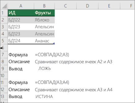
Сравнение одной ячейки с другой
Для этого используйте функцию СОВСХ.
Примечание: Функция СОВПАД учитывает регистр, но игнорирует различия в форматировании.
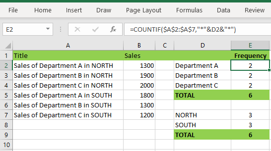
Сравнение одного значения со списком значений
Для этого используйте функции СОВКА и ИЛИ.
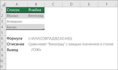
Примечание: Если у вас установлена текущая версия Microsoft 365, можно просто ввести формулу в верхней левой ячейке диапазона вывода и нажать клавишу ВВОД, чтобы подтвердить использование формулы динамического массива. В противном случае формулу необходимо ввести как формулу массива прежних вариантов: сначала выберем ячейку, введите формулу в ячейку вывода, а затем нажимая CTRL+SHIFT+ВВОД, чтобы подтвердить ее. Excel автоматически вставляет фигурные скобки в начале и конце формулы. Дополнительные сведения о формулах массива см. в статье Использование формул массива: рекомендации и примеры.
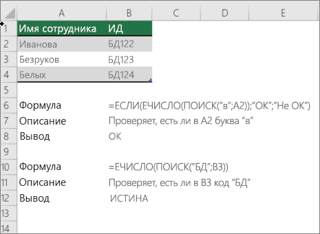
Проверка того, совпадает ли часть ячейки с определенным текстом
Для этого используйте функции ЕСЛИ,НАЙТИ иЕ ЧИСЛОЭЛЕБР.
Примечание: Функция НАЙТИ работает с чувствительностью к делу.
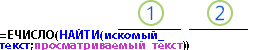
В формуле на снимке экрана выше используются следующие аргументы:
Формула для поиска текста
-
search_for: что вы хотите проверить.
-
to_search:ячейка с текстом, который нужно проверить.
Нужна дополнительная помощь?
Excel has a number of formulas that help you use your data in useful ways. For example, you can get an output based on whether or not a cell meets certain specifications. Right now, we’ll focus on a function called “if cell contains, then”. Let’s look at an example.
Jump To Specific Section:
- Explanation: If Cell Contains
- If cell contains any value, then return a value
- If cell contains text/number, then return a value
- If cell contains specific text, then return a value
- If cell contains specific text, then return a value (case-sensitive)
- If cell does not contain specific text, then return a value
- If cell contains one of many text strings, then return a value
- If cell contains several of many text strings, then return a value
Excel Formula: If cell contains
Generic formula
=IF(ISNUMBER(SEARCH("abc",A1)),A1,"")
Summary
To test for cells that contain certain text, you can use a formula that uses the IF function together with the SEARCH and ISNUMBER functions. In the example shown, the formula in C5 is:
=IF(ISNUMBER(SEARCH("abc",B5)),B5,"")
If you want to check whether or not the A1 cell contains the text “Example”, you can run a formula that will output “Yes” or “No” in the B1 cell. There are a number of different ways you can put these formulas to use. At the time of writing, Excel is able to return the following variations:
- If cell contains any value
- If cell contains text
- If cell contains number
- If cell contains specific text
- If cell contains certain text string
- If cell contains one of many text strings
- If cell contains several strings
Using these scenarios, you’re able to check if a cell contains text, value, and more.
Explanation: If Cell Contains
One limitation of the IF function is that it does not support Excel wildcards like «?» and «*». This simply means you can’t use IF by itself to test for text that may appear anywhere in a cell.
One solution is a formula that uses the IF function together with the SEARCH and ISNUMBER functions. For example, if you have a list of email addresses, and want to extract those that contain «ABC», the formula to use is this:
=IF(ISNUMBER(SEARCH("abc",B5)),B5,""). Assuming cells run to B5
If «abc» is found anywhere in a cell B5, IF will return that value. If not, IF will return an empty string («»). This formula’s logical test is this bit:
ISNUMBER(SEARCH("abc",B5))
Read article: Excel efficiency: 11 Excel Formulas To Increase Your Productivity
Using “if cell contains” formulas in Excel
The guides below were written using the latest Microsoft Excel 2019 for Windows 10. Some steps may vary if you’re using a different version or platform. Contact our experts if you need any further assistance.
1. If cell contains any value, then return a value
This scenario allows you to return values based on whether or not a cell contains any value at all. For example, we’ll be checking whether or not the A1 cell is blank or not, and then return a value depending on the result.
- Select the output cell, and use the following formula: =IF(cell<>»», value_to_return, «»).
- For our example, the cell we want to check is A2, and the return value will be No. In this scenario, you’d change the formula to =IF(A2<>»», «No», «»).
- Since the A2 cell isn’t blank, the formula will return “No” in the output cell. If the cell you’re checking is blank, the output cell will also remain blank.
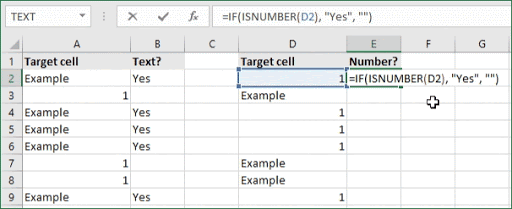
2. If cell contains text/number, then return a value
With the formula below, you can return a specific value if the target cell contains any text or number. The formula will ignore the opposite data types.
Check for text
- To check if a cell contains text, select the output cell, and use the following formula: =IF(ISTEXT(cell), value_to_return, «»).
- For our example, the cell we want to check is A2, and the return value will be Yes. In this scenario, you’d change the formula to =IF(ISTEXT(A2), «Yes», «»).

- Because the A2 cell does contain text and not a number or date, the formula will return “Yes” into the output cell.
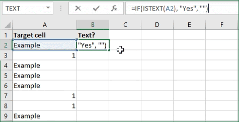
Check for a number or date
- To check if a cell contains a number or date, select the output cell, and use the following formula: =IF(ISNUMBER(cell), value_to_return, «»).
- For our example, the cell we want to check is D2, and the return value will be Yes. In this scenario, you’d change the formula to =IF(ISNUMBER(D2), «Yes», «»).

- Because the D2 cell does contain a number and not text, the formula will return “Yes” into the output cell.
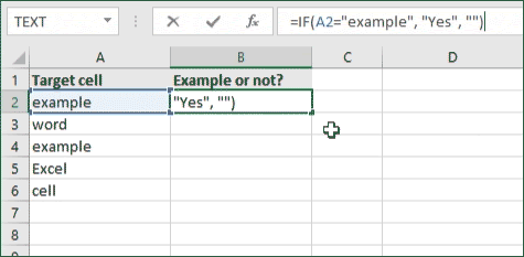
3. If cell contains specific text, then return a value
To find a cell that contains specific text, use the formula below.
- Select the output cell, and use the following formula: =IF(cell=»text», value_to_return, «»).
- For our example, the cell we want to check is A2, the text we’re looking for is “example”, and the return value will be Yes. In this scenario, you’d change the formula to =IF(A2=»example», «Yes», «»).

- Because the A2 cell does consist of the text “example”, the formula will return “Yes” into the output cell.
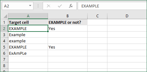
4. If cell contains specific text, then return a value (case-sensitive)
To find a cell that contains specific text, use the formula below. This version is case-sensitive, meaning that only cells with an exact match will return the specified value.
- Select the output cell, and use the following formula: =IF(EXACT(cell,»case_sensitive_text»), «value_to_return», «»).
- For our example, the cell we want to check is A2, the text we’re looking for is “EXAMPLE”, and the return value will be Yes. In this scenario, you’d change the formula to =IF(EXACT(A2,»EXAMPLE»), «Yes», «»).
- Because the A2 cell does consist of the text “EXAMPLE” with the matching case, the formula will return “Yes” into the output cell.
5. If cell does not contain specific text, then return a value
The opposite version of the previous section. If you want to find cells that don’t contain a specific text, use this formula.
- Select the output cell, and use the following formula: =IF(cell=»text», «», «value_to_return»).
- For our example, the cell we want to check is A2, the text we’re looking for is “example”, and the return value will be No. In this scenario, you’d change the formula to =IF(A2=»example», «», «No»).
- Because the A2 cell does consist of the text “example”, the formula will return a blank cell. On the other hand, other cells return “No” into the output cell.
6. If cell contains one of many text strings, then return a value
This formula should be used if you’re looking to identify cells that contain at least one of many words you’re searching for.
- Select the output cell, and use the following formula: =IF(OR(ISNUMBER(SEARCH(«string1», cell)), ISNUMBER(SEARCH(«string2», cell))), value_to_return, «»).
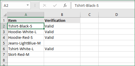
- For our example, the cell we want to check is A2. We’re looking for either “tshirt” or “hoodie”, and the return value will be Valid. In this scenario, you’d change the formula to =IF(OR(ISNUMBER(SEARCH(«tshirt»,A2)),ISNUMBER(SEARCH(«hoodie»,A2))),»Valid «,»»).
- Because the A2 cell does contain one of the text values we searched for, the formula will return “Valid” into the output cell.
To extend the formula to more search terms, simply modify it by adding more strings using ISNUMBER(SEARCH(«string», cell)).
7. If cell contains several of many text strings, then return a value
This formula should be used if you’re looking to identify cells that contain several of the many words you’re searching for. For example, if you’re searching for two terms, the cell needs to contain both of them in order to be validated.
- Select the output cell, and use the following formula: =IF(AND(ISNUMBER(SEARCH(«string1»,cell)), ISNUMBER(SEARCH(«string2″,cell))), value_to_return,»»).
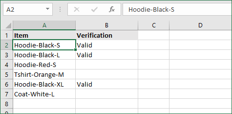
- For our example, the cell we want to check is A2. We’re looking for “hoodie” and “black”, and the return value will be Valid. In this scenario, you’d change the formula to =IF(AND(ISNUMBER(SEARCH(«hoodie»,A2)),ISNUMBER(SEARCH(«black»,A2))),»Valid «,»»).
- Because the A2 cell does contain both of the text values we searched for, the formula will return “Valid” to the output cell.
Final thoughts
We hope this article was useful to you in learning how to use “if cell contains” formulas in Microsoft Excel. Now, you can check if any cells contain values, text, numbers, and more. This allows you to navigate, manipulate and analyze your data efficiently.
We’re glad you’re read the article up to here  Thank you
You may also like
» How to use NPER Function in Excel
» How to Separate First and Last Name in Excel
» How to Calculate Break-Even Analysis in Excel
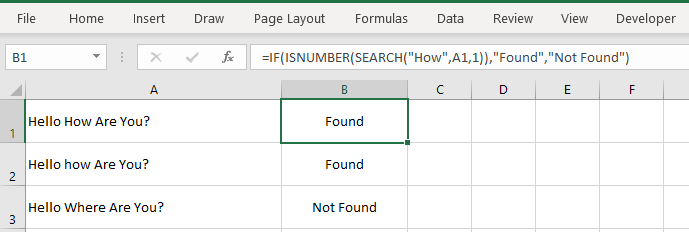
In this example, the goal is to test a value in a cell to see if it contains a specific substring. Excel contains two functions designed to check the occurrence of one text string inside another: the SEARCH function and the FIND function. Both functions return the position of the substring if found as a number, and a #VALUE! error if the substring is not found. The difference is that the SEARCH function supports wildcards but is not case-sensitive, while the FIND function is case-sensitive but does not support wildcards. The general approach with either function is to use the ISNUMBER function to check for a numeric result (a match) and return TRUE or FALSE.
SEARCH function (not case-sensitive)
The SEARCH function is designed to look inside a text string for a specific substring. If SEARCH finds the substring, it returns a position of the substring in the text as a number. If the substring is not found, SEARCH returns a #VALUE error. For example:
=SEARCH("p","apple") // returns 2
=SEARCH("z","apple") // returns #VALUE!
To force a TRUE or FALSE result, we use the ISNUMBER function. ISNUMBER returns TRUE for numeric values and FALSE for anything else. So, if SEARCH finds the substring, it returns the position as a number, and ISNUMBER returns TRUE:
=ISNUMBER(SEARCH("p","apple")) // returns TRUE
=ISNUMBER(SEARCH("z","apple")) // returns FALSE
If SEARCH doesn’t find the substring, it returns an error, which causes the ISNUMBER to return FALSE.
Wildcards
Although SEARCH is not case-sensitive, it does support wildcards (*?~). For example, the question mark (?) wildcard matches any one character. The formula below looks for a 3-character substring beginning with «x» and ending in «y»:
=ISNUMBER(SEARCH("x?z","xyz")) // TRUE
=ISNUMBER(SEARCH("x?z","xbz")) // TRUE
=ISNUMBER(SEARCH("x?z","xyy")) // FALSE
The asterisk (*) wildcard matches zero or more characters. This wildcard is not as useful in the SEARCH function because SEARCH already looks for a substring. For example, it might seem like the following formula will test for a value that ends with «z»:
=ISNUMBER(SEARCH("*z",text))However, because SEARCH automatically looks for a substring, the following formulas all return 1 as a result, even though the text in the first formula is the only text that ends with «z»:
=SEARCH("*z","XYZ") // returns 1
=SEARCH("*z","XYZXY") // returns 1
=SEARCH("*z","XYZXY123") // returns 1
=SEARCH("x*z","XYZXY123") // returns 1
This means the asterisk (*) is not a reliable way to test for «ends with». However, you an use the the asterisk (*) wildcard like this:
=SEARCH("x*2*b","AAAXYZ123ABCZZZ") // returns 4
=SEARCH("x*2*b","NXYZ12563JKLB") // returns 2
Here we are looking for «x», «2», and «b» in that order, with any number of characters in between. Finally, you can use the tilde (~) as an escape character to indicate that the next character is a literal like this:
=SEARCH("~*","apple*") // returns 6
=SEARCH("~?","apple?") // returns 6
=SEARCH("~~","apple~") // returns 6
The above formulas use SEARCH to find a literal asterisk (*), question mark (?) , and tilde (~) in that order.
FIND function (case-sensitive)
Like the SEARCH function, the FIND function returns the position of a substring in text as a number, and an error if the substring is not found. However, unlike the SEARCH function, the FIND function respects case:
=FIND("A","Apple") // returns 1
=FIND("A","apple") // returns #VALUE!
To make a case-sensitive version of the formula, just replace the SEARCH function with the FIND function in the formula above:
=ISNUMBER(FIND(substring,A1))
The result is a case-sensitive search:
=ISNUMBER(FIND("A","Apple")) // returns TRUE
=ISNUMBER(FIND("A","apple")) // returns FALSE
If cell contains
To return a custom result when a cell contains specific text, add the IF function like this:
=IF(ISNUMBER(SEARCH(substring,A1)), "Yes", "No")
Instead of returning TRUE or FALSE, the formula above will return «Yes» if substring is found and «No» if not.
With hardcoded search string
To test for a hardcoded substring, enclose the text in double quotes («»). For example, to check A1 for the text «apple» use:
=ISNUMBER(SEARCH("apple",A1))
More than one search string
To test a cell for more than one thing (i.e. for one of many substrings), see this example formula.
 Наверное, многие задавались вопросом, как найти функцию в EXCEL«СОДЕРЖИТ», чтобы применить какое-либо условие, в зависимости от того, есть ли в текстовой строке кусок слова, или отрицание, или часть наименования контрагента, особенно при нестандартном заполнении реестров вручную.
Такой функционал возможно получить с помощью сочетания двух обычных стандартных функций – ЕСЛИ и СЧЁТЕСЛИ.
Рассмотрим пример автоматизации учета операционных показателей на основании реестров учета продаж и возвратов (выгрузки из сторонних программ автоматизации и т.п.)
У нас есть множество строк с документами Реализации и Возвратов.
Все документы имеют свое наименование за счет уникального номера.
Нам необходимо сделать признак «Только реализация» напротив документов продажи, для того, чтобы в дальнейшем включить этот признак в сводную таблицу и исключить возвраты для оценки эффективности деятельности отдела продаж.
Выражение должно быть универсальным, для того, чтобы обрабатывать новые добавляемые данные.
Для того, чтобы это сделать, необходимо:
- Начинаем с ввода функции ЕСЛИ (вводим «=», набираем наименование ЕСЛИ, выбираем его из выпадающего списка, нажимаем fx в строке формул).

- В открывшемся окне аргументов, в поле Лог_выражение вводим СЧЁТЕСЛИ(), выделяем его и нажимаем 2 раза fx.
- Далее в открывшемся окне аргументов функции СЧЁТЕСЛИ в поле «Критерий» вводим кусок искомого наименования *реализ*, добавляя в начале и в конце символ *.
Такая запись даст возможность не думать о том, с какой стороны написано слово реализация (до или после номера документа), а также даст возможность включить в расчет сокращенные слова «реализ.» и «реализац.»
- Аргумент «Диапазон» — это соответствующая ячейка с наименованием документа.
- Далее нажимаем ОК, выделяем в строке формул ЕСЛИ и нажимаем fx и продолжаем заполнение функции ЕСЛИ.
- В Значение_если_истина вводим «Реализация», а в Значение_если_ложь – можно ввести прочерк « — »
- Далее протягиваем формулу до конца таблицы и подключаем сводную.
Теперь мы можем работать и сводить данные только по документам реализации исключая возвраты. При дополнении таблицы новыми данными, остается только протягивать строку с нашим выражением и обновлять сводную таблицу.
Если материал Вам понравился или даже пригодился, Вы можете поблагодарить автора, переведя определенную сумму по кнопке ниже:
(для перевода по карте нажмите на VISA и далее «перевести»)
На чтение 9 мин Просмотров 12.3к. Опубликовано 31.07.2020
Содержание
- Функция ЕСЛИ СОДЕРЖИТ
- Проверяем условие для полного совпадения текста.
- ЕСЛИ + СОВПАД
- Использование функции ЕСЛИ с частичным совпадением текста.
- ЕСЛИ + ПОИСК
- ЕСЛИ + НАЙТИ
- Функция ЕСЛИ: примеры с несколькими условиями
- Если ячейки не пустые, то делаем расчет
- Проверка ввода данных в Excel
- Функция ЕСЛИ: проверяем условия с текстом
- Визуализация данных при помощи функции ЕСЛИ
- Как функция ЕСЛИ работает с датами?
- Функция ЕСЛИ в Excel – примеры использования
- Поиск ячеек, содержащих текст
- Проверка ячейки на наличие в ней текста
- Проверка соответствия ячейки определенному тексту
- Проверка соответствия части ячейки определенному тексту
Функция ЕСЛИ СОДЕРЖИТ
Наверное, многие задавались вопросом, как найти функцию в EXCEL«СОДЕРЖИТ» , чтобы применить какое-либо условие, в зависимости от того, есть ли в текстовой строке кусок слова , или отрицание, или часть наименования контрагента, особенно при нестандартном заполнении реестров вручную.
Такой функционал возможно получить с помощью сочетания двух обычных стандартных функций – ЕСЛИ и СЧЁТЕСЛИ .
Рассмотрим пример автоматизации учета операционных показателей на основании реестров учета продаж и возвратов (выгрузки из сторонних программ автоматизации и т.п.)
У нас есть множество строк с документами Реализации и Возвратов .
Все документы имеют свое наименование за счет уникального номера .
Нам необходимо сделать признак « Только реализация » напротив документов продажи, для того, чтобы в дальнейшем включить этот признак в сводную таблицу и исключить возвраты для оценки эффективности деятельности отдела продаж.
Выражение должно быть универсальным , для того, чтобы обрабатывать новые добавляемые данные .
Для того, чтобы это сделать, необходимо:
-
- Начинаем с ввода функции
ЕСЛИ
-
- (вводим
«=»
-
- , набираем наименование
ЕСЛИ
-
- , выбираем его из выпадающего списка, нажимаем
fx
-
- в строке формул).

В открывшемся окне аргументов, в поле Лог_выражение вводим СЧЁТЕСЛИ() , выделяем его и нажимаем 2 раза fx.

Далее в открывшемся окне аргументов функции СЧЁТЕСЛИ в поле «Критерий» вводим кусок искомого наименования *реализ* , добавляя в начале и в конце символ * .

Такая запись даст возможность не думать о том, с какой стороны написано слово реализация (до или после номера документа), а также даст возможность включить в расчет сокращенные слова «реализ.» и «реализац.»
- Аргумент «Диапазон» — это соответствующая ячейка с наименованием документа.
- Далее нажимаем ОК , выделяем в строке формул ЕСЛИ и нажимаем fx и продолжаем заполнение функции ЕСЛИ.

- В Значение_если_истина вводим « Реализация », а в Значение_если_ложь – можно ввести прочерк « — »
- Далее протягиваем формулу до конца таблицы и подключаем сводную.


Теперь мы можем работать и сводить данные только по документам реализации исключая возвраты . При дополнении таблицы новыми данными, остается только протягивать строку с нашим выражением и обновлять сводную таблицу.
Если материал Вам понравился или даже пригодился, Вы можете поблагодарить автора, переведя определенную сумму по кнопке ниже:
(для перевода по карте нажмите на VISA и далее «перевести»)
Рассмотрим использование функции ЕСЛИ в Excel в том случае, если в ячейке находится текст.
Будьте особо внимательны в том случае, если для вас важен регистр, в котором записаны ваши текстовые значения. Функция ЕСЛИ не проверяет регистр – это делают функции, которые вы в ней используете. Поясним на примере.
Проверяем условие для полного совпадения текста.
Проверку выполнения доставки организуем при помощи обычного оператора сравнения «=».
=ЕСЛИ(G2=»выполнено»,ИСТИНА,ЛОЖЬ)
При этом будет не важно, в каком регистре записаны значения в вашей таблице.

Если же вас интересует именно точное совпадение текстовых значений с учетом регистра, то можно рекомендовать вместо оператора «=» использовать функцию СОВПАД(). Она проверяет идентичность двух текстовых значений с учетом регистра отдельных букв.
Вот как это может выглядеть на примере.

Обратите внимание, что если в качестве аргумента мы используем текст, то он обязательно должен быть заключён в кавычки.
ЕСЛИ + СОВПАД
В случае, если нас интересует полное совпадение текста с заданным условием, включая и регистр его символов, то оператор «=» нам не сможет помочь.
Но мы можем использовать функцию СОВПАД (английский аналог — EXACT).
Функция СОВПАД сравнивает два текста и возвращает ИСТИНА в случае их полного совпадения, и ЛОЖЬ — если есть хотя бы одно отличие, включая регистр букв. Поясним возможность ее использования на примере.
Формула проверки выполнения заказа в столбце Н может выглядеть следующим образом:

Как видите, варианты «ВЫПОЛНЕНО» и «выполнено» не засчитываются как правильные. Засчитываются только полные совпадения. Будет полезно, если важно точное написание текста — например, в артикулах товаров.
Использование функции ЕСЛИ с частичным совпадением текста.
Выше мы с вами рассмотрели, как использовать текстовые значения в функции ЕСЛИ. Но часто случается, что необходимо определить не полное, а частичное совпадение текста с каким-то эталоном. К примеру, нас интересует город, но при этом совершенно не важно его название.
Первое, что приходит на ум – использовать подстановочные знаки «?» и «*» (вопросительный знак и звездочку). Однако, к сожалению, этот простой способ здесь не проходит.
ЕСЛИ + ПОИСК
Нам поможет функция ПОИСК (в английском варианте – SEARCH). Она позволяет определить позицию, начиная с которой искомые символы встречаются в тексте. Синтаксис ее таков:
=ПОИСК(что_ищем, где_ищем, начиная_с_какого_символа_ищем)
Если третий аргумент не указан, то поиск начинаем с самого начала – с первого символа.
Функция ПОИСК возвращает либо номер позиции, начиная с которой искомые символы встречаются в тексте, либо ошибку.
Но нам для использования в функции ЕСЛИ нужны логические значения.
Здесь нам на помощь приходит еще одна функция EXCEL – ЕЧИСЛО. Если ее аргументом является число, она возвратит логическое значение ИСТИНА. Во всех остальных случаях, в том числе и в случае, если ее аргумент возвращает ошибку, ЕЧИСЛО возвратит ЛОЖЬ.
В итоге наше выражение в ячейке G2 будет выглядеть следующим образом:
Еще одно важное уточнение. Функция ПОИСК не различает регистр символов.

ЕСЛИ + НАЙТИ
В том случае, если для нас важны строчные и прописные буквы, то придется использовать вместо нее функцию НАЙТИ (в английском варианте – FIND).
Синтаксис ее совершенно аналогичен функции ПОИСК: что ищем, где ищем, начиная с какой позиции.
Изменим нашу формулу в ячейке G2

То есть, если регистр символов для вас важен, просто замените ПОИСК на НАЙТИ.
Итак, мы с вами убедились, что простая на первый взгляд функция ЕСЛИ дает нам на самом деле много возможностей для операций с текстом.
Примеры использования функции ЕСЛИ:

Функция ЕСЛИ: примеры с несколькими условиями
Для того, чтобы описать условие в функции ЕСЛИ, Excel позволяет использовать более сложные конструкции. В том числе можно использовать и несколько условий. Рассмотрим на примере. Для объединения нескольких условий в […]

Если ячейки не пустые, то делаем расчет
Чтобы выполнить действие только тогда, когда ячейка не пуста (содержит какие-то значения), вы можете использовать формулу, основанную на функции ЕСЛИ. В примере ниже столбец F содержит даты завершения закупок шоколада. […]

Проверка ввода данных в Excel
Подтверждаем правильность ввода галочкой. Задача: При ручном вводе данных в ячейки таблицы проверять правильность ввода в соответствии с имеющимся списком допустимых значений. В случае правильного ввода в отдельном столбце ставить […]
Функция ЕСЛИ: проверяем условия с текстом
Рассмотрим использование функции ЕСЛИ в Excel в том случае, если в ячейке находится текст. Будьте особо внимательны в том случае, если для вас важен регистр, в котором записаны ваши текстовые […]
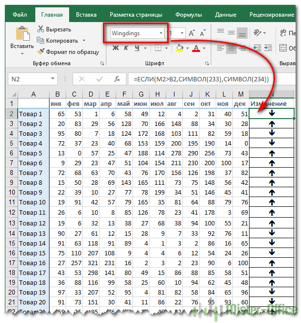
Визуализация данных при помощи функции ЕСЛИ
Функцию ЕСЛИ можно использовать для вставки в таблицу символов, которые наглядно показывают происходящие с данными изменения. К примеру, мы хотим показать, происходит рост или снижение продаж. В столбце N поставим […]
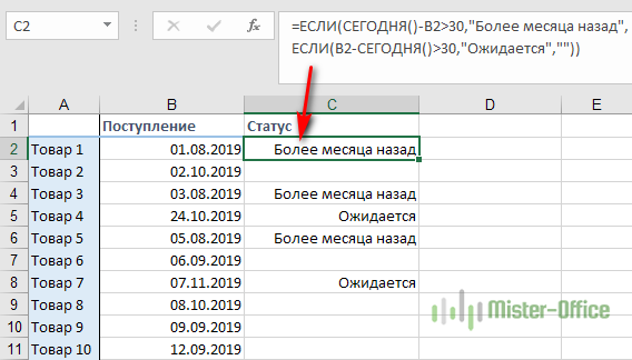
Как функция ЕСЛИ работает с датами?
На первый взгляд может показаться, что функцию ЕСЛИ для работы с датами можно использовать так же, как для числовых и текстовых значений, которые мы только что обсудили. К сожалению, это […]

Функция ЕСЛИ в Excel – примеры использования
на примерах рассмотрим, как можно использовать функцию ЕСЛИ в Excel, а также какие задачи мы можем решить с ее помощью
Примечание: Мы стараемся как можно оперативнее обеспечивать вас актуальными справочными материалами на вашем языке. Эта страница переведена автоматически, поэтому ее текст может содержать неточности и грамматические ошибки. Для нас важно, чтобы эта статья была вам полезна. Просим вас уделить пару секунд и сообщить, помогла ли она вам, с помощью кнопок внизу страницы. Для удобства также приводим ссылку на оригинал (на английском языке).
Допустим, вы хотите убедиться, что столбец имеет текст, а не числа. Или перхапсйоу нужно найти все заказы, соответствующие определенному продавцу. Если вы не хотите учитывать текст верхнего или нижнего регистра, есть несколько способов проверить, содержит ли ячейка.
Вы также можете использовать фильтр для поиска текста. Дополнительные сведения можно найти в разделе Фильтрация данных.
Поиск ячеек, содержащих текст
Чтобы найти ячейки, содержащие определенный текст, выполните указанные ниже действия.
Выделите диапазон ячеек, которые вы хотите найти.
Чтобы выполнить поиск на всем листе, щелкните любую ячейку.
На вкладке Главная в группе Редактирование нажмите кнопку найти _амп_и выберите пункт найти.
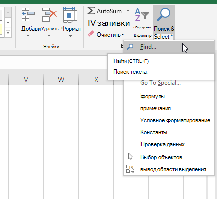
В поле найти введите текст (или числа), который нужно найти. Вы также можете выбрать последний поисковый запрос из раскрывающегося списка найти .
Примечание: В критериях поиска можно использовать подстановочные знаки.
Чтобы задать формат поиска, нажмите кнопку Формат и выберите нужные параметры в всплывающем окне Найти формат .
Нажмите кнопку Параметры , чтобы еще больше задать условия поиска. Например, можно найти все ячейки, содержащие данные одного типа, например формулы.
В поле внутри вы можете выбрать лист или книгу , чтобы выполнить поиск на листе или во всей книге.
Нажмите кнопку найти все или Найти далее.
Найдите все списки всех вхождений элемента, который нужно найти, и вы можете сделать ячейку активной, выбрав определенное вхождение. Вы можете отсортировать результаты поиска » найти все «, щелкнув заголовок.
Примечание: Чтобы остановить поиск, нажмите клавишу ESC.
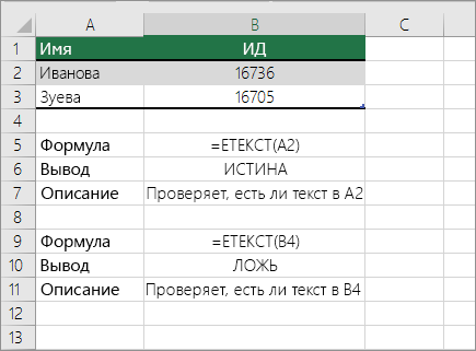
Проверка ячейки на наличие в ней текста
Для выполнения этой задачи используйте функцию текст .
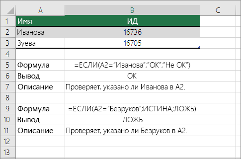
Проверка соответствия ячейки определенному тексту
Используйте функцию Если , чтобы вернуть результаты для указанного условия.
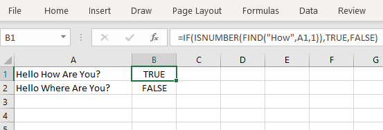
Проверка соответствия части ячейки определенному тексту
Для выполнения этой задачи используйте функции Если, Поиски функция номер .
Примечание: Функция Поиск не учитывает регистр.
Здесь в руководстве представлены формулы, позволяющие проверить, содержит ли ячейка определенный текст и вернуть значение ИСТИНА и ЛОЖЬ, как показано на скриншоте ниже, а также объясняются аргументы и принцип работы формул.
Формула 1 Проверка, содержит ли ячейка определенный текст (без учета регистра)
Общая формула:
=ISNUMBER(SEARCH(substring,text))
аргументы
| Substring: the specific text you want to search in the cell. |
| Text: the cell or text string you want to check if contains a specific text (the argument substring) |
Возвращаемое значение:
Эта формула возвращает логическое значение. Если ячейка содержит подстроку, формула возвращает ИСТИНА или ЛОЖЬ.
Как работает эта формула
Здесь вы хотите проверить, содержит ли ячейка B3 текст в C3, используйте формулу ниже
Нажмите Enter ключ для получения результата проверки.
объяснение
ПОИСК функция: функция ПОИСК возвращает позицию первого символа find_text во внутри_text, если она не находит find_text, она вернет #VALUE! значение ошибки. Вот ПОИСК (C3, B3) найдет позицию текста в ячейке C3 внутри ячейки B3, вернет 22.
Функция ISNUMBER: функция ISNUMBER проверяет, является ли значение в ячейке числовым значением, и возвращает логическое значение. Возвращение TRUE указывает, что ячейка содержит числовое значение, или возвращает FALSE. Вот ISNUMBER (ПОИСК (C3, B3)) проверит, является ли результат функции ПОИСК числовым значением.
Формула 2 Проверить, содержит ли ячейка определенный текст (с учетом регистра)
Общая формула:
=ISNUMBER(FIND(substring,text))
аргументы
| Substring: the specific text you want to search in the cell. |
| Text: the cell or text string you want to check if contains a specific text (the argument substring). |
Возвращаемое значение:
Эта формула возвращает логическое значение. Если ячейка содержит подстроку, формула возвращает ИСТИНА или ЛОЖЬ.
Как работает эта формула
Здесь вы хотите проверить, содержит ли ячейка B4 текст в C4, используйте формулу ниже
Нажмите Enter ключ для проверки.
объяснение
НАЙТИ функция: функция НАЙТИ получает местоположение первого символа find_text в пределах_text, если она не находит find_text, она вернет #VALUE! значение ошибки, и оно чувствительно к регистру. Вот НАЙТИ (C4; B4) найдет позицию текста в ячейке C4 внутри ячейки B4 и вернет #VALUE! значение ошибки ..
Функция ISNUMBER: функция ISNUMBER проверяет, является ли значение в ячейке числовым значением, и возвращает логическое значение. Возвращение TRUE указывает, что ячейка содержит числовое значение, или возвращает FALSE. Вот ЕЧИСЛО (НАЙТИ (C4; B4)) проверит, является ли результат функции НАЙТИ числовым значением.
Файл примера
 Нажмите, чтобы загрузить образец файла
Относительные формулы
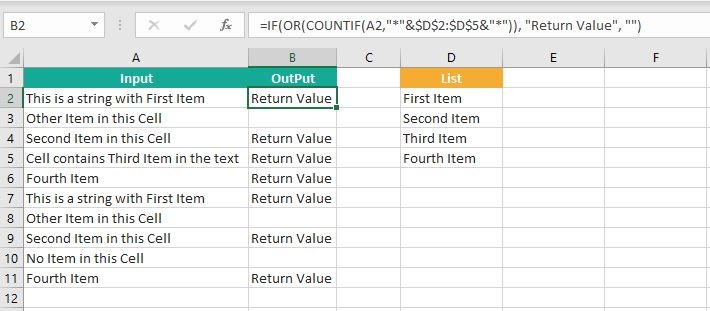
- Проверьте, содержит ли ячейка одно из множества значений
В этом руководстве представлена формула, позволяющая проверить, содержит ли ячейка одно из нескольких значений в Excel, а также объясняются аргументы в формуле и принцип работы формулы. - Проверить, содержит ли ячейка одно из нескольких значений, но исключить другие значения
В этом руководстве будет представлена формула для быстрого решения задачи, которая проверяет, содержит ли ячейка одно из элементов, но исключает другие значения в Excel, и объясняет аргументы формулы. - Проверьте, содержит ли ячейка что-либо из
Предположим, что в Excel есть список значений в столбце E, вы хотите проверить, содержат ли ячейки в столбце B все значения в столбце E, и вернуть TRUE или FALSE. - Проверить, содержит ли ячейка номер
Иногда вам может потребоваться проверить, содержит ли ячейка числовые символы. В этом руководстве представлена формула, которая вернет ИСТИНА, если ячейка содержит число, и ЛОЖЬ, если ячейка не содержит числа.
Лучшие инструменты для работы в офисе
Kutools for Excel — Помогает вам выделиться из толпы
Хотите быстро и качественно выполнять свою повседневную работу? Kutools for Excel предлагает 300 мощных расширенных функций (объединение книг, суммирование по цвету, разделение содержимого ячеек, преобразование даты и т. д.) и экономит для вас 80 % времени.
- Разработан для 1500 рабочих сценариев, помогает решить 80% проблем с Excel.
- Уменьшите количество нажатий на клавиатуру и мышь каждый день, избавьтесь от усталости глаз и рук.
- Станьте экспертом по Excel за 3 минуты. Больше не нужно запоминать какие-либо болезненные формулы и коды VBA.
- 30-дневная неограниченная бесплатная пробная версия. 60-дневная гарантия возврата денег. Бесплатное обновление и поддержка 2 года.
")
Вкладка Office — включение чтения и редактирования с вкладками в Microsoft Office (включая Excel)
- Одна секунда для переключения между десятками открытых документов!
- Уменьшите количество щелчков мышью на сотни каждый день, попрощайтесь с рукой мыши.
- Повышает вашу продуктивность на 50% при просмотре и редактировании нескольких документов.
- Добавляет эффективные вкладки в Office (включая Excel), точно так же, как Chrome, Firefox и новый Internet Explorer.
")
Комментарии (0)
Оценок пока нет. Оцените первым!
![]()
Excel If Cell Contains Text

Excel If Cell Contains Text Then Formula helps you to return the output when a cell have any text or a specific text. You can check if a cell contains a some string or text and produce something in other cell. For Example you can check if a cell A1 contains text ‘example text’ and print Yes or No in Cell B1. Following are the example Formulas to check if Cell contains text then return some thing in a Cell.
If Cell Contains Text
Here are the Excel formulas to check if Cell contains specific text then return something. This will return if there is any string or any text in given Cell. We can use this simple approach to check if a cell contains text, specific text, string, any text using Excel If formula. We can use equals to operator(=) to compare the strings .
If Cell Contains Text Then TRUE
Following is the Excel formula to return True if a Cell contains Specif Text. You can check a cell if there is given string in the Cell and return True or False.
The formula will return true if it found the match, returns False of no match found.
If Cell Contains Partial Text
We can return Text If Cell Contains Partial Text. We use formula or VBA to Check Partial Text in a Cell.
Find for Case Sensitive Match:
We can check if a Cell Contains Partial Text then return something using Excel Formula. Following is a simple example to find the partial text in a given Cell. We can use if your want to make the criteria case sensitive.
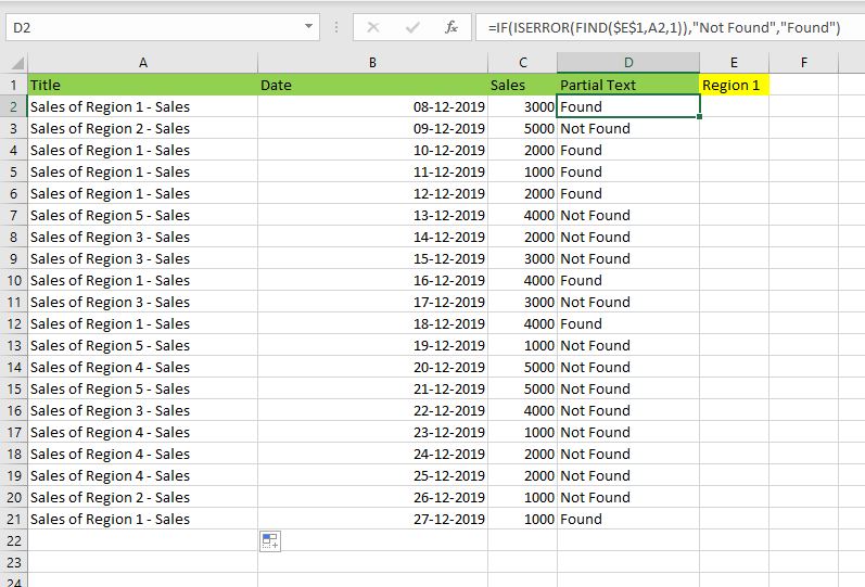
- Here, Find Function returns the finding position of the given string
- Use Find function is Case Sensitive
- IsError Function check if Find Function returns Error, that means, string not found
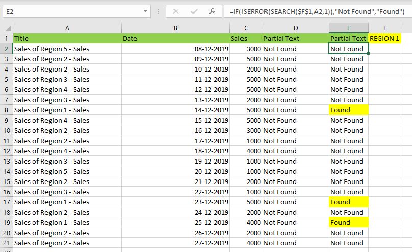
Search for Not Case Sensitive Match:
We can use Search function to check if Cell Contains Partial Text. Search function useful if you want to make the checking criteria Not Case Sensitive.
If Range of Cells Contains Text
We can check for the strings in a range of cells. Here is the formula to find If Range of Cells Contains Text. We can use Count If Formula to check the excel if range of cells contains specific text and return Text.
- CountIf function counts the number of cells with given criteria
- We can use If function to return the required Text
- Formula displays the Text ‘Range Contains Text” if match found
- Returns “Text Not Found in the Given Range” if match not found in the specified range
If Cells Contains Text From List
Below formulas returns text If Cells Contains Text from given List. You can use based on your requirement.
VlookUp to Check If Cell Contains Text from a List:
We can use VlookUp function to match the text in the Given list of Cells. And return the corresponding values.
- Check if a List Contains Text:
=IF(ISERR(VLOOKUP(F1,A1:B21,2,FALSE)),”False:Not Contains”,”True: Text Found”) - Check if a List Contains Text and Return Corresponding Value:
=VLOOKUP(F1,A1:B21,2,FALSE) - Check if a List Contains Partial Text and Return its Value:
=VLOOKUP(“*”&F1&”*”,A1:B21,2,FALSE)
If Cell Contains Text Then Return a Value
We can return some value if cell contains some string. Here is the the the Excel formula to return a value if a Cell contains Text. You can check a cell if there is given string in the Cell and return some string or value in another column.
The formula will return true if it found the match, returns False of no match found. can
Excel if cell contains word then assign value
You can replace any word in the following formula to check if cell contains word then assign value.
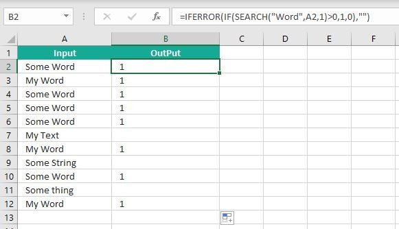
Search function will check for a given word in the required cell and return it’s position. We can use If function to check if the value is greater than 0 and assign a given value (example: 1) in the cell. search function returns #Value if there is no match found in the cell, we can handle this using IFERROR function.
Count If Cell Contains Text
We can check If Cell Contains Text Then COUNT. Here is the Excel formula to Count if a Cell contains Text. You can count the number of cells containing specific text.
The formula will Sum the values in Column B if the cells of Column A contains the given text.
Count If Cell Contains Partial Text
We can count the cells based on partial match criteria. The following Excel formula Counts if a Cell contains Partial Text.
- We can use the CountIf Function to Count the Cells if they contains given String
- Wild-card operators helps to make the CountIf to check for the Partial String
- Put Your Text between two asterisk symbols (*YourText*) to make the criteria to find any where in the given Cell
- Add Asterisk symbol at end of your text (YourText*) to make the criteria to find your text beginning of given Cell
- Place Asterisk symbol at beginning of your text (*YourText) to make the criteria to find your text end of given Cell
If Cell contains text from list then return value
Here is the Excel Formula to check if cell contains text from list then return value. We can use COUNTIF and OR function to check the array of values in a Cell and return the given Value. Here is the formula to check the list in range D2:D5 and check in Cell A2 and return value in B2.
If Cell Contains Text Then SUM
Following is the Excel formula to Sum if a Cell contains Text. You can total the cell values if there is given string in the Cell. Here is the example to sum the column B values based on the values in another Column.
The formula will Sum the values in Column B if the cells of Column A contains the given text.

Sum If Cell Contains Partial Text
Use SumIfs function to Sum the cells based on partial match criteria. The following Excel formula Sums the Values if a Cell contains Partial Text.
- SUMIFS Function will Sum the Given Sum Range
- We can specify the Criteria Range, and wild-card expression to check for the Partial text
- Put Your Text between two asterisk symbols (*YourText*) to Sum the Cells if the criteria to find any where in the given Cell
- Add Asterisk symbol at end of your text (YourText*) to Sum the Cells if the criteria to find your text beginning of given Cell
- Place Asterisk symbol at beginning of your text (*YourText) to Sum the Cells if criteria to find your text end of given Cell
VBA to check if Cell Contains Text
Here is the VBA function to find If Cells Contains Text using Excel VBA Macros.
If Cell Contains Partial Text VBA
We can use VBA to check if Cell Contains Text and Return Value. Here is the simple VBA code match the partial text. Excel VBA if Cell contains partial text macros helps you to use in your procedures and functions.
MsgBox CheckIfCellContainsPartialText(Cells(2, 1), “Region 1”)
End Sub
Function CheckIfCellContainsPartialText(ByVal cell As Range, ByVal strText As String) As Boolean
If InStr(1, cell.Value, strText) > 0 Then CheckIfCellContainsPartialText = True
End Function
- CheckIfCellContainsPartialText VBA Function returns true if Cell Contains Partial Text
- inStr Function will return the Match Position in the given string
If Cell Contains Text Then VBA MsgBox
Here is the simple VBA code to display message box if cell contains text. We can use inStr Function to search for the given string. And show the required message to the user.
If InStr(1, Cells(2, 1), “Region 3”) > 0 Then blnMatch = True
If blnMatch = True Then MsgBox “Cell Contains Text”
End Sub
- inStr Function will return the Match Position in the given string
- blnMatch is the Boolean variable becomes True when match string
- You can display the message to the user if a Range Contains Text
Which function returns true if cell a1 contains text?
You can use the Excel If function and Find function to return TRUE if Cell A1 Contains Text. Here is the formula to return True.
Which function returns true if cell a1 contains text value?
You can use the Excel If function with Find function to return TRUE if a Cell A1 Contains Text Value. Below is the formula to return True based on the text value.
Share This Story, Choose Your Platform!
7 Comments
-
Meghana
December 27, 2019 at 1:42 pm — ReplyHi Sir,Thank you for the great explanation, covers everything and helps use create formulas if cell contains text values.
Many thanks! Meghana!!
-
Max
December 27, 2019 at 4:44 pm — ReplyPerfect! Very Simple and Clear explanation. Thanks!!
-
Mike Song
August 29, 2022 at 2:45 pm — ReplyI tried this exact formula and it did not work.
-
Theresa A Harding
October 18, 2022 at 9:51 pm — Reply -
Marko
November 3, 2022 at 9:21 pm — ReplyHi
Is possible to sum all WA11?
(A1) WA11 4
(A2) AdBlue 1, WA11 223
(A3) AdBlue 3, WA11 32, shift 4
… and everything is in one column.
Thanks you very much for your help.
Sincerely Marko
-
Mike
December 9, 2022 at 9:59 pm — ReplyThank you for the help. The formula =OR(COUNTIF(M40,”*”&Vendors&”*”)) will give “TRUE” when some part of M40 contains a vendor from “Vendors” list. But how do I get Excel to tell which vendor it found in the M40 cell?
-
PNRao
December 18, 2022 at 6:05 am — ReplyPlease describe your question more elaborately.
Thanks!
-
© Copyright 2012 – 2020 | Excelx.com | All Rights Reserved
Page load link
You can use the following formula in Excel to determine if a cell contains a certain string:
=IF(ISNUMBER(SEARCH("this",A1)), "Yes", "No")
In this example, if cell A1 contains the string “this” then it will return a Yes, otherwise it will return a No.
The following examples show how to use this formula in practice.
Example: Check if Cell Contains a Certain String in Excel
Suppose we have the following dataset in Excel that shows the number of points scored by various basketball players:

We can use the following formula to check if the value in the Team column contains the string “mavs”:
=IF(ISNUMBER(SEARCH("mavs",A2)), "Yes", "No")
We can type this formula into cell C2 and then copy and paste it down to the remaining cells in column C:

The three rows with a value of “mavs” in the Team column all receive a Yes in the new column while all other rows receive a No.
Note that the SEARCH() function in Excel is case-insensitive.
If you’d like to perform a case-sensitive search, you can swap out the SEARCH() function in the formula with the FIND() function.
For example, we could use the following formula to check if any value in the Team column is equal to “MAVS”:
=IF(ISNUMBER(FIND("MAVS",A2)), "Yes", "No")
The following screenshot shows how to use this formula in practice:

Notice that every value in the new column is equal to No because none of the team names match the uppercase “MAVS” string that we specified in the formula.
Additional Resources
The following tutorials explain how to perform other common tasks in Excel:
How to Count Duplicates in Excel
How to Count Frequency of Text in Excel
How to Calculate Average If Cell Contains Text in Excel