
![]()
Symbols Used in Excel Formula

Here are the important symbols used in Excel Formulas. Each of these special characters have used for different purpose in Excel. Let us see complete list of symbols used in Excel Formulas, its meaning and uses.
Symbols used in Excel Formula
Following symbols are used in Excel Formula. They will perform different actions in Excel Formulas and Functions.
| Symbol | Name | Description |
|---|---|---|
| = | Equal to | Every Excel Formula begins with Equal to symbol (=).
Example:=A1+A5 |
| () | Parentheses | All Arguments of the Excel Functions specified between the Parentheses.
Example:=COUNTIF(A1:A5,5) |
| () | Parentheses | Expressions specified in the Parentheses will be evaluated first. Parentheses changes the order of the evaluation in Excel Formula.
Example: =25+(35*2)+5 |
| * | Asterisk | Wild card operator to to denote all values in a List.
Example: =COUNTIF(A1:A5,”*“) |
| , | Comma | List of the Arguments of a Function Separated by Comma in Excel Formula.
Example: =COUNTIF(A1:A5,“>” &B1) |
| & | Ampersand | Concatenate Operator to connect two strings into one in Excel Formula.
Example: =”Total: “&SUM(B2:B25) |
| $ | Dollar | Makes Cell Reference as Absolute in Excel Formula.
Example:=SUM($B$2:$B$25) |
| ! | Exclamation | Sheet Names and Table Names Followed by ! Symbol in Excel Formula.
Example: =SUM(Sheet2!B2:B25) |
| [] | Square Brackets | Uses to refer the Field Name of the Table (List Object) in Excel Formula.
Example:=SUM(Table1[Column1]) |
| {} | Curly Brackets | Denote the Array formula in Excel.
Example: {=MAX(A1:A5-G1:G5)} |
| : | Colon | Creates references to all cells between two references.
Example: =SUM(B2:B25) |
| , | Comma | Union Operator will combine the multiple references into One.
Example: =SUM(A2:A25, B2:B25) |
| (space) | Space | Intersection Operator will create common reference of two references.
Example: =SUM(A2:A10 A5:A25) |
Share This Story, Choose Your Platform!
6 Comments
-
Redjen
May 31, 2022 at 12:37 pm — Replywhat is the symbol of average in excel?
-
PNRao
June 20, 2022 at 12:40 pm — ReplyYou can use AVERAGE()Function to calculate Average in Excel. If you wants to show the Average Statistical Symbol (x-bar), You can insert from symbols. F7C2 is the Unicode Hexa character for X-bar symbol. Make sure that you have set the Symbol Font :MS Reference Sans Serif.
-
-
Tom Pearce
September 22, 2022 at 3:54 pm — ReplyI have a workbook, where the original author used an @ sign in front of a function call in a formula. I can find no reference as to what the @ does, or how it is used. Any one know??
VBA Example: ActiveSheet.Range(“L2”).Formula = “=@CATEGORY($E2,LFC_AreaLU)”
Note: Category is a User Defined Function in the workbook.-
PNRao
December 5, 2022 at 11:30 am — Reply
-
-
Jane Girard
February 9, 2023 at 8:53 pm — ReplyI have this formula, do you know what the al means in the formula ?
IF(E4=””,””,VLOOKUP(C4,al,5,0)*E4), can-
PNRao
February 27, 2023 at 3:10 am — ReplyIt could be a defined Name or a name of the Table (List Object)
-
© Copyright 2012 – 2020 | Excelx.com | All Rights Reserved
Page load link
Содержание
- Functions CHAR SIGN TYPE in Excel and examples of their formulas
- Examples of using the CHAR, TYPE and SIGN functions in excel formulas
- How to count the number of positive and negative numbers in Excel
- Checking what types of cell input data in an Excel spreadsheet
- How to use a wildcard in Excel formula
- How to use a wildcard in Excel formula
- Wildcard
- Available wildcards
- Example wildcard usage
- Functions that support wildcards
- Excel Wildcard Characters – What are these and How to Best Use it
- Excel Wildcard Characters – An Introduction
- Excel Wildcard Characters – Examples
- #1 Filter Data using Excel Wildcard Characters
- #2 Partial Lookup Using Wildcard Characters & VLOOKUP
- 3. Find and Replace Partial Matches
- 4. Count Non-blank Cells that Contain Text
Functions CHAR SIGN TYPE in Excel and examples of their formulas
In Excel, it is often necessary to use when calculating values that are tied to symbols, the sign of a number, and the type.
The following functions are used for this:
CHAR function makes it possible to get a character with its given code. The function is used to convert the numeric character codes that are received from other computers into characters of the given computer.
TYPE function determines the data types of the cell, returning the corresponding number.
SIGN function returns the sign of a number and returns the value 1 if it is positive, 0 if it is 0, and -1 if it is negative.
Examples of using the CHAR, TYPE and SIGN functions in excel formulas
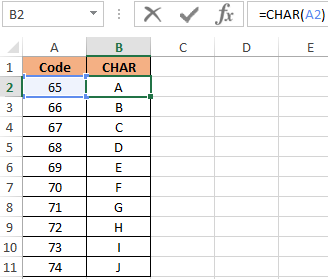
Example 1. Given a table with character codes: from 65 — to 74:
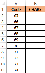
It is necessary with the help of the CHAR to display the characters that correspond to these codes.
To do this, we enter into the cell B2 the following formula:
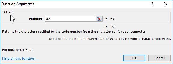
The function argument: Number is the character code.
As a result of the calculations we get:
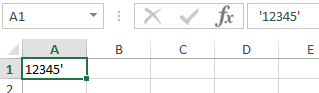
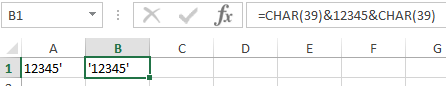
How to use the CHAR in formulas in practice? For example, we need to display a text string in single quotes. For Excel, a single quote as the first character is a special character that converts any cell value to a text data type. Therefore, in the cell itself, the single quote as the first character is not displayed:
To solve this problem, we use the following formula with the function =CHAR(39)
It is also useful to use this function when you need to make a line break in an Excel cell as a formula. And for other similar tasks.
The value 39 in the function argument, you guessed it, is the character code of a single quote.
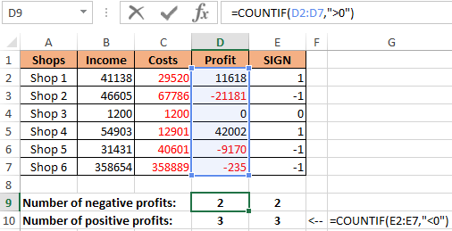
How to count the number of positive and negative numbers in Excel
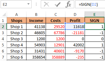
Example 2. The table contains 3 numbers. Calculate which character has each number: positive (+), negative (-) or 0.
Let’s enter the data in the table of the form:
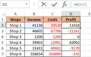
We introduce the formula in cell E2:
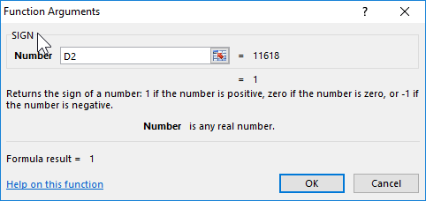
Argument: Number — any real numeric value.
By copying this formula down, we get:
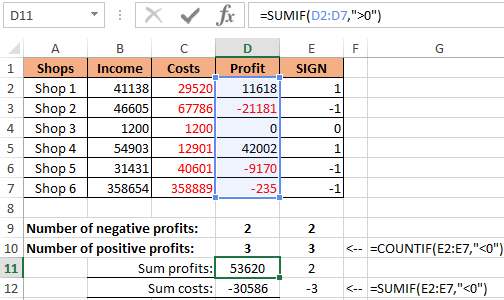
First, we calculate the number of negative and positive numbers in the columns «Profit» and «SIGN»:
And now we summarize only positive or only negative numbers:
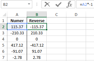
How to make a negative number positive and positive negative? It is very simple to multiply by -1:
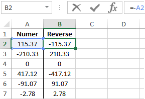
You can even simplify the formula, simply put a subtraction operator sign — minus, before the cell reference:
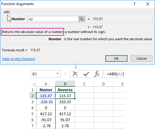
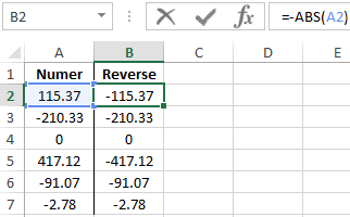
But what if you need to make a number with any sign positive? Then you should use the ABS function. This function returns any number by module:
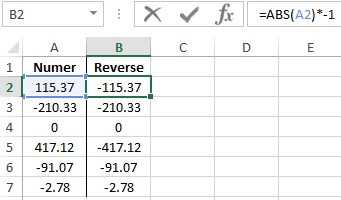
Now it is not difficult to guess how to make any number with a negative minus sign:
Checking what types of cell input data in an Excel spreadsheet
Example 3. Using the TYPE function, display the type of data that is entered in the table:
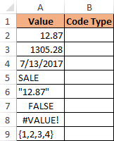
TYPE function returns the code of the data types that can be entered into an Excel cell:
| Data Value | Type Code |
| number | 1 |
| text | 2 |
| logical value | 4 |
| error value | 16 |
| array | 64 |
We introduce the formula for the calculation in cell B2:
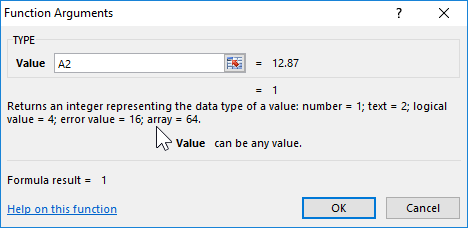
Argument: Value is any valid value.
As a result, we get:
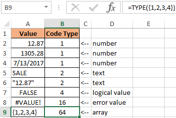
Thus, using the TYPE function, you can always check what the Excel cell actually contains. Note that the date is defined by the function as a number. For Excel, any date is a numeric value that corresponds to the number of days that have passed from January 01/01/1900, to the original date. Therefore, each date in Excel should be taken as a numeric data type displayed in the cell format — “Date”.
Источник
How to use a wildcard in Excel formula

Excel supports wildcard characters in formulas to find values that share a simple pattern. For example, if you are looking for a string with known ending or beginning, and unknown characters in the middle, you can use wildcard characters to tell Excel to look for all compatible matches. In this article, we’re going to show you how to use a wildcard in Excel formula.
How to use a wildcard in Excel formula
In total, there are 3 wildcard characters you can use in Excel. You can use 2 of them as a replacement of characters, and the third one to prevent the other 2 from being registered as wildcard characters.
- ? character stands for a single character. For example, X-M?n finds both X-Men and X-Man.
- * character stands for one or more characters. For example, s*man finds both Spider-Man and Superman
character that followed by ?, *,
characters searches the following character without using it as a wildcard. For example, X-M
?n finds only X-M?n.
All characters can be used in conjunction. For example, s*??n text finds Spawn, as well as Spider-Man and Superman.
You can use wildcard characters inside various functions. In the example bewlo, we used the VLOOKUP function to find the name of the publisher of a fictional character that ends with «boy«. To find a text that ends with «boy«, we used an asterisk (*) as a replacement for any characters before «boy«. ;
Below is a list of formulas you can use with wildcards.
- AVERAGEIF
- AVERAGEIFS
- COUNTIF
- COUNTIFS
- HLOOKUP
- MATCH
- SEARCH
- SUMIF
- SUMIFS
- VLOOKUP
Источник
Wildcard
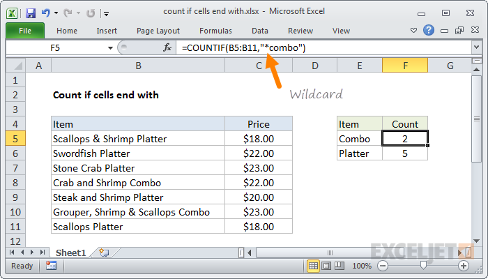
A wildcard is a special character that lets you perform «fuzzy» matching on text in your Excel formulas. For example, this formula:
counts all cells in the range B5:B11 that end with the text «combo». And this formula:
Counts all cells in A1:A100 that contain exactly 3 characters.
Available wildcards
Excel has 3 wildcards you can use in your formulas:
- Asterisk (*) — zero or more characters
- Question mark (?) — any one character
- Tilde (
) — escape for literal character (
*) a literal question mark (
?), or a literal tilde (
Example wildcard usage
| Usage | Behavior | Will match |
|---|---|---|
| ? | Any one character | «A», «B», «c», «z», etc. |
| ?? | Any two characters | «AA», «AZ», «zz», etc. |
| . | Any three characters | «Jet», «AAA», «ccc», etc. |
| * | Any characters | «apple», «APPLE», «A100», etc. |
| *th | Ends in «th» | «bath», «fourth», etc. |
| c* | Starts with «c» | «Cat», «CAB», «cindy», «candy», etc. |
| ?* | At least one character | «a», «b», «ab», «ABCD», etc. |
| . -?? | 5 characters with hypen | «ABC-99″,»100-ZT», etc. |
| * |
? Ends in question mark «Hello?», «Anybody home?», etc. *xyz* Contains «xyz» «code is XYZ», «100-XYZ», «XyZ90», etc.
Wildcards only work with text. For numeric data, you can use logical operators.
Functions that support wildcards
Not all functions allow wildcards. Here is a list of the most common functions that do:
Источник
Excel Wildcard Characters – What are these and How to Best Use it
Watch Video on Excel Wildcard Characters
There are only 3 Excel wildcard characters (asterisk, question mark, and tilde) and a lot can be done using these.
In this tutorial, I will show you four examples where these Excel wildcard characters are absolute lifesavers.
This Tutorial Covers:
Excel Wildcard Characters – An Introduction
Wildcards are special characters that can take any place of any character (hence the name – wildcard).
There are three wildcard characters in Excel:
- * (asterisk) – It represents any number of characters . For example, Ex* could mean Excel, Excels, Example, Expert, etc.
- ? (question mark) – It represents one single character. For example, Tr?mp could mean Trump or Tramp.
(tilde) – It is used to identify a wildcard character (
, *, ?) in the text. For example, let’s say you want to find the exact phrase Excel* in a list. If you use Excel* as the search string, it would give you any word that has Excel at the beginning followed by any number of characters (such as Excel, Excels, Excellent). To specifically look for excel*, we need to use
. So our search string would be excel
*. Here, the presence of
ensures that excel reads the following character as is, and not as a wildcard.
Note: I have not come across many situations where you need to use
. Nevertheless, it is a good to know feature.
Now let’s go through four awesome examples where wildcard characters do all the heavy lifting.
Excel Wildcard Characters – Examples
Now let’s look at four practical examples where Excel wildcard characters can be mighty useful:
- Filtering data using a wildcard character.
- Partial Lookup using wildcard character and VLOOKUP.
- Find and Replace Partial Matches.
- Count Non-blank cells that contain text.
#1 Filter Data using Excel Wildcard Characters
Excel wildcard characters come in handy when you have huge data sets and you want to filter data based on a condition.
Suppose you have a dataset as shown below:

You can use the asterisk (*) wildcard character in data filter to get a list of companies that start with the alphabet A.
Here is how to do this:
This will instantly filter the results and give you 3 names – ABC Ltd., Amazon.com, and Apple Stores.

How does it work? – When you add an asterisk (*) after A, Excel would filter anything that starts with A. This is because an asterisk (being an Excel wildcard character) can represent any number of characters.
Now with the same methodology, you can use various criteria to filter results.
For example, if you want to filter companies that begin with the alphabet A and contain the alphabet C in it, use the string A*C. This will give you only 2 results – ABC Ltd. and Amazon.com.
If you use A?C instead, you will only get ABC Ltd as the result (as only one character is allowed between ‘a’ and ‘c’)
#2 Partial Lookup Using Wildcard Characters & VLOOKUP
Partial look-up is needed when you have to look for a value in a list and there isn’t an exact match.
For example, suppose you have a data set as shown below, and you want to look for the company ABC in a list, but the list has ABC Ltd instead of ABC.
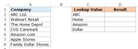
You can not use the regular VLOOKUP function in this case as the lookup value does not have an exact match.
If you use VLOOKUP with an approximate match, it will give you the wrong results.
However, you can use a wildcard character within VLOOKUP function to get the right results:
Enter the following formula in cell D2 and drag it for other cells:
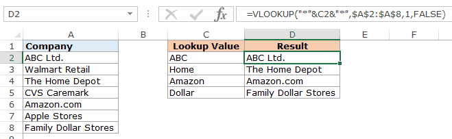
How does this formula work?
In the above formula, instead of using the lookup value as is, it is flanked on both sides with the Excel wildcard character asterisk (*) – “*”&C2&”*”
This tells excel that it needs to look for any text that contains the word in C2. It could have any number of characters before or after the text in C2.
Hence, the formula looks for a match, and as soon as it gets a match, it returns that value.
3. Find and Replace Partial Matches
Excel Wildcard characters are quite versatile.
You can use it in a complex formula as well as in basic functionality such as Find and Replace.
Suppose you have the data as shown below:

In the above data, the region has been entered in different ways (such as North-West, North West, NorthWest).
This is often the case with sales data.
To clean this data and make it consistent, we can use Find and Replace with Excel wildcard characters.
Here is how to do this:
- Select the data where you want to find and replace text.
- Go to Home –> Find & Select –> Go To. This will open the Find and Replace dialogue box. (You can also use the keyboard shortcut – Control + H).
- Enter the following text in the find and replace dialogue box:
- Find what: North*W*
- Replace with: North-West

- Click on Replace All.

This will instantly change all the different formats and make it consistent to North-West.

How does this Work?
In the Find field, we have used North*W* which will find any text that has the word North and contains the alphabet ‘W’ anywhere after it.
Hence, it covers all the scenarios (NorthWest, North West, and North-West).
Find and Replace finds all these instances and changes it to North-West and makes it consistent.
4. Count Non-blank Cells that Contain Text
I know you are smart and you thinking that Excel already has an inbuilt function to do this.
You’re absolutely right!!
This can be done using the COUNTA function.
BUT… There is one small problem with it.
A lot of times when you import data or use other people’s worksheet, you will notice that there are empty cells while that might not be the case.
These cells look blank but have =”” in it. The trouble is that the
The trouble is that the COUNTA function does not consider this as an empty cell (it counts it as text).
See the example below:

In the above example, I use the COUNTA function to find cells that are not empty and it returns 11 and not 10 (but you can clearly see only 10 cells have text).
The reason, as I mentioned, is that it doesn’t consider A11 as empty (while it should).
But that is how Excel works.
The fix is to use the Excel wildcard character within the formula.
Below is a formula using the COUNTIF function that only counts cells that have text in it:
This formula tells excel to count only if the cell has at least one character.
In the ?* combo:
- ? (question mark) ensures that at least one character is present.
- * (asterisk) makes room for any number of additional characters.
Note: The above formula works when only have text values in the cells. If you have a list that has both text as well as numbers, use the following formula:
Similarly, you can use wildcards in a lot of other Excel functions, such as IF(), SUMIF(), AVERAGEIF(), and MATCH().
It’s also interesting to note that while you can use the wildcard characters in the SEARCH function, you can’t use it in FIND function.
Hope these examples give you a flair of the versatility and power of Excel wildcard characters.
If you have any other innovative way to use it, do share it with me in the comments section.
You May Find the Following Excel Tutorials Useful:
Источник
Excel for Microsoft 365 Excel for Microsoft 365 for Mac Excel for the web Excel 2021 Excel 2021 for Mac Excel 2019 Excel 2019 for Mac Excel 2016 Excel 2016 for Mac Excel 2013 More…Less
We often hear that you want to make data easier to understand by including text in your formulas, such as «2,347 units sold.» To include text in your functions and formulas, surround the text with double quotes («»). The quotes tell Excel it’s dealing with text, and by text, we mean any character, including numbers, spaces, and punctuation. Here’s an example:
=A2&» sold «&B2&» units.»
For this example, pretend the cells in column A contain names, and the cells in column B contain sales numbers. The result would be something like: Buchanan sold 234 units.
The formula uses ampersands (&) to combine the values in columns A and B with the text. Also, notice how the quotes don’t surround cell B2. They enclose the text that comes before and after the cell.
Here’s another example of a common task, adding the date to worksheet. It uses the TEXT and TODAY functions to create a phrase such as «Today is Friday, January 20.»
=»Today is » & TEXT(TODAY(),»dddd, mmmm dd.»)
Let’s see how this one works from the inside out. The TODAY function calculates today’s date, but it displays a number, such as 40679. The TEXT function then converts the number to a readable date by first changing the number to text, and then using «dddd, mmmm dd» to control how the date appears—«Friday, January 20.»
Make sure you surround «ddd, mmmm dd» date format with double quotes, and notice how the format uses commas and spaces. Normally, formulas use commas to separate the arguments—the pieces of data—they need to run. But when you treat commas as text, you can use them whenever you need to.
Finally, the formula uses the & to combine the formatted date with the words «Today is «. And yes, put a space after the «is.»
Need more help?
Want more options?
Explore subscription benefits, browse training courses, learn how to secure your device, and more.
Communities help you ask and answer questions, give feedback, and hear from experts with rich knowledge.
Hello friends,
In this article, I am going to explain you, how can you use special characters in Excel VBA and formulas without breaking the syntax.
For Example: You can not use double quote or any other Special Characters, which are generally a part of Formula Syntax, directly in a cell while using formula because using them, will spoil the syntax of the formula and it will through an error. To overcome this issue, one can use the ASCII number of those characters. ASCII values can be used to refer the characters in both Excel formulas as well as Excel VBA.
Use of ASCII numbers in Excel Formulas as well as Excel VBA programming
Excel Formulas
CHAR( ASCII Number)
Excel VBA
VBA.Chr( ASCII Number)
Here is the list of ASCII keys of few most used symbols which may affect the formula syntax in Excel if they are used as it is:
| Symbol | ASCII Code | Syntax – Excel Formula | Syntax – Excel VBA |
|---|---|---|---|
| $ – Dollar Sign | 36 | =Char(36) | VBA.Chr(36) |
| ” – Double Quote | 34 | =Char(34) | VBA.Chr(34) |
| & – Ampersand Sign | 38 | =Char(38) | VBA.Chr(38) |
| ( – Opening Braces | 40 | =Char(40) | VBA.Chr(40) |
| ) – Closing Braces | 41 | =Char(41) | VBA.Chr(41) |
| @ – At the rate Sign | 64 | =Char(64) | VBA.Chr(64) |
A wildcard is a special character that lets you perform «fuzzy» matching on text in your Excel formulas. For example, this formula:
=COUNTIF(B5:B11,"*combo")
counts all cells in the range B5:B11 that end with the text «combo». And this formula:
=COUNTIF(A1:A100,"???")
Counts all cells in A1:A100 that contain exactly 3 characters.
Available wildcards
Excel has 3 wildcards you can use in your formulas:
- Asterisk (*) — zero or more characters
- Question mark (?) — any one character
- Tilde (~) — escape for literal character (~*) a literal question mark (~?), or a literal tilde (~~).
Note: wildcards only work with text, not numbers.
Example wildcard usage
| Usage | Behavior | Will match |
|---|---|---|
| ? | Any one character | «A», «B», «c», «z», etc. |
| ?? | Any two characters | «AA», «AZ», «zz», etc. |
| ??? | Any three characters | «Jet», «AAA», «ccc», etc. |
| * | Any characters | «apple», «APPLE», «A100», etc. |
| *th | Ends in «th» | «bath», «fourth», etc. |
| c* | Starts with «c» | «Cat», «CAB», «cindy», «candy», etc. |
| ?* | At least one character | «a», «b», «ab», «ABCD», etc. |
| ???-?? | 5 characters with hypen | «ABC-99″,»100-ZT», etc. |
| *~? | Ends in question mark | «Hello?», «Anybody home?», etc. |
| *xyz* | Contains «xyz» | «code is XYZ», «100-XYZ», «XyZ90», etc. |
Wildcards only work with text. For numeric data, you can use logical operators.
More general information on formula criteria here.
Functions that support wildcards
Not all functions allow wildcards. Here is a list of the most common functions that do:
- AVERAGEIF, AVERAGEIFS
- COUNTIF, COUNTIFS
- MAXIFS, MINIFS
- SUMIF, SUMIFS
- VLOOKUP, HLOOKUP
- MATCH
- SEARCH