Microsoft Excel is used for performing to the simple mathematical operations. The true functionality of the program is much broader.
Excel allows you to solve very complex problems, to perform unique mathematical calculations, to analyze statistical data and much more. The important element of the working field in Microsoft Excel is the formula bar. Let’s try to understand the principles of its work and answer to the key questions that related to it.
What is the purpose of the Formula Bar in Excel?
The Microsoft Excel is one of the most useful programs that allows by the user to perform more than 400 mathematical operations. All of them are grouped into 9 categories:
- financial;
- date and time;
- text;
- the statistics;
- mathematical;
- arrays and links;
- the work with BD;
- brain teaser;
- the verification of values, properties and characteristics.
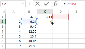
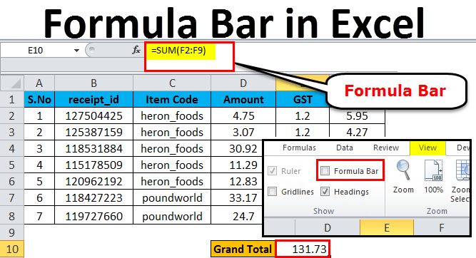
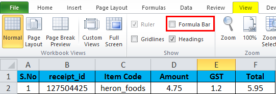
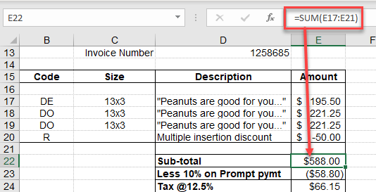
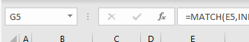
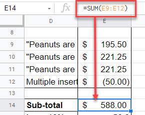
All these functions can be easily tracked in the cells and edited thanks to the formula bar. It displays everything that each cell contains. In the picture it is highlighted in red.
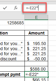
Entering the sign «=» in it, you seem to «activate» the bar and tell to the program that you are going to enter some data, formulas.
How to enter the formula in a string?
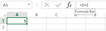
The formulas can be entered into the cells manually or using the formula bar. For writing the formula in the cell, you need to start it with the «=» sign. For example, you need to enter data into our cell A1. To do this we select it, put the «=» sign and enter the data. The line «will come to working condition» by itself. For example, we took the same cell «A1», entered the sign «=» and pressed the input for calculating to the sum of two numbers.
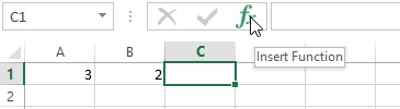
You can use the function wizard (fx button):
- We to activate the required cell and go to the formula bar, find the «fx» icon and click in it.
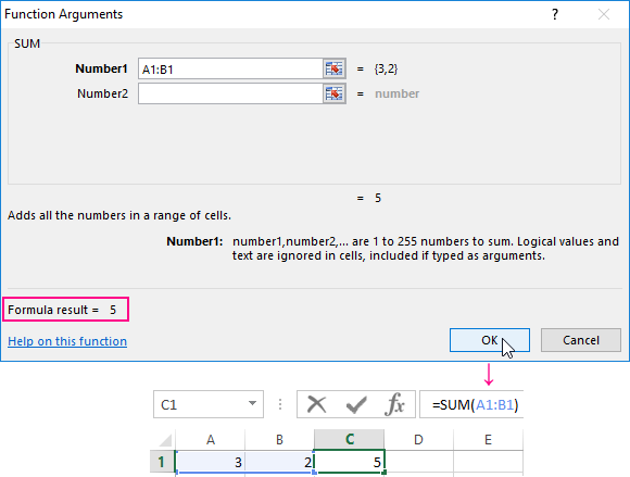
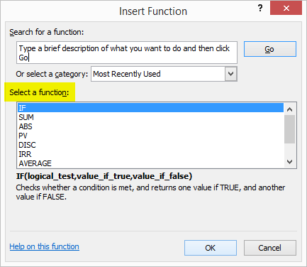
- It suggests immediately to choose the function =SUM(), that is necessary for the user. We select the desired option and click «OK».
- Next in the dialog box we enter the values in the parameters of the selected function.
What does the Excel formula editor line contain? In practice, in this field you can:
- to enter the numbers and text from the keyboard;
- to specify the references to the ranges of cells;
- to edit the function arguments.
IMPORTANT! There is the list of typical errors that occur after an error entry, in such case the system will refuse to perform the calculation. Instead, it will give you strange values at first glance. That they were not for you cause of panic, we give their decoding.
- «#LINK!». It says, that you specified an incorrect reference to one cell or to the range of cells;
- «#NAME?». Check if you entered the correct cell address and the function name;
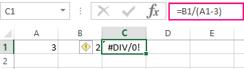
- «# DEL! / 0!». It says about the prohibition of division by 0. Most likely, you entered the cell with a «zero» value in the formula string;
- «#NUMBER!». It evidences, that the value of the argument of the function does not match the allowable value;
- «##########». The width of your cell is not enough to display the resulting number. You need to expand it.
All these errors are displayed in the cells, and the value in the formula line is stored after input.
What does the $ sign mean in Excel Formula Bar?
Users need to copy the formula so often, inserting it into another place of the working field. The problem is that when copying or filling out the form, the link is adjusted automatically. Therefore, you can not even «hinder» by the automatic process of the replacing the addresses of links in the copied formulas. There are relative references, that are written without the signs «$».
The $ sign is used to leave addresses for links in the formula parameters unchanged when it is copied or populated. The absolute reference is prescribed with two signs of «$»: before the letter (the column header) and in front of the figure (the title of the line). This is how the absolute link looks like: = $C$1.
The mixed link allows you to leave the value of a column or a string unchanged. If you put the «$» before the letter in the formula, then the value of the row number.
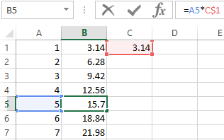
But if the formula shifts relative to the columns (horizontally), then the link will change, as it is mixed.
The using mixed links allows you to vary formulas and values.
The note. In order not to switch the layout every time you look for the «$» sign, you need to use the F4 key to enter the address. It serves as the link type switch. If you press it periodically, the symbol «$» is inserted automatically, making the links absolute or mixed.
The formula string was missing in Excel
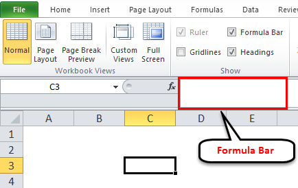
How to return a string of formulas in Excel in place? The most common reason of its disappearance – is the changing of settings. Most likely, you accidentally pressed something, and this led to the disappearance of the line. To return it and continue working with documents, it is necessary to perform the following sequence of the actions:
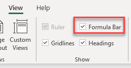
- To select the tab labeled «View» on the panel and click on it.
- To check, if the tick next to the «Formula Bar» is checked. If it does not exist, we set it.
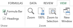
After that, the missing line in the program «returns» to the place it was assigned. In the same way, you can remove it, if necessary.
One more option. Go to the settings «File» – «Options» – «Advanced». In the right list of settings, we find the «Screen» section in the same place and check the «Show Formula Bar» option.
The Large Formula Bar
The line for entering data into the cells can be increased if you can not see a large and complex formula entirely. For this:
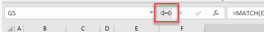
- Hover your mouse over the border between the line and the column headings of the sheet so, that it changes its appearance to 2 arrows.
- While holding to the left mouse button, move the cursor down to the required number of lines, until the content is displayed freely.
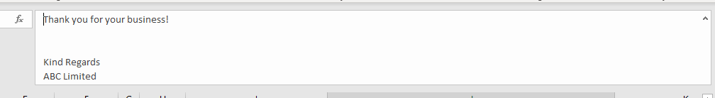
Thus, you can see and edit long functions. Also this method is useful for those cells, that contain a lot of text information.
Formula Bar in Excel (Table of Contents)
- What is Formula Bar in Excel?
- How to Use Formula Bar in Excel?
- How to Use Formula Bar Icons?
- How to Expand the Visibility of Formula Bar?
- How to Protect the Formula from Unwanted Editing?
What is Formula Bar in Excel?
Formula Bar in Excel is a section where we can see values and formulas stored in it. The Formula generally is already seen below the menu bar. But if it is not there, then we can activate this from the View menu option under the Show section. It can also be activated from the Excel Option’s Advanced tab. Apart from showing the values and formula of any cell, Formula Bar also tells at which cell we have kept the cursor and the Insert Function option denoted by fx.
The content of the current cell or where the selection is pointed will be visible in the formula bar. Visibility includes:
- Current cell selection.
- The formula applied in the active cell.
- The range of cells selected in the excel.
How to Use Formula Bar in Excel?
The formula bar can be used to edit the content of any cell and can be expanded to show multiple lines for the same formula. Let’s understand the function with a few examples.
You can download this Formula Bar Excel Template here – Formula Bar Excel Template
Formula Bar in Excel – Example #1
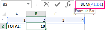
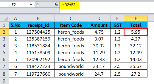
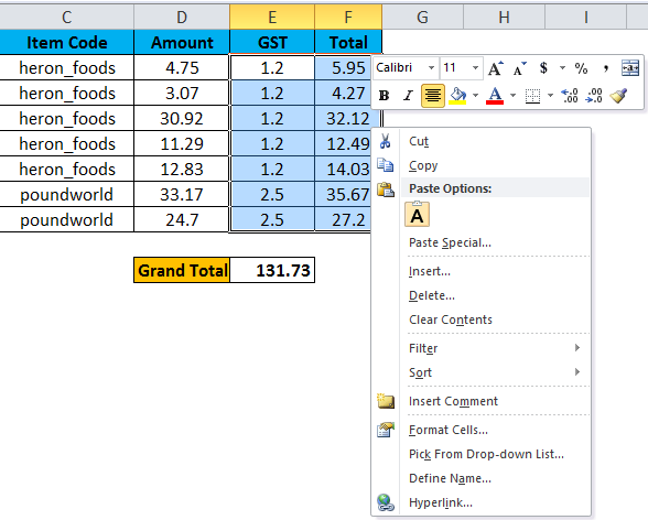
The formula applied for the total column is the sum of the amount and GST. The formula “=D2+E2” is applied to the entire column. The formula applied within the formula bar is visible, and the corresponding cells are filed with the value after applying the formula.
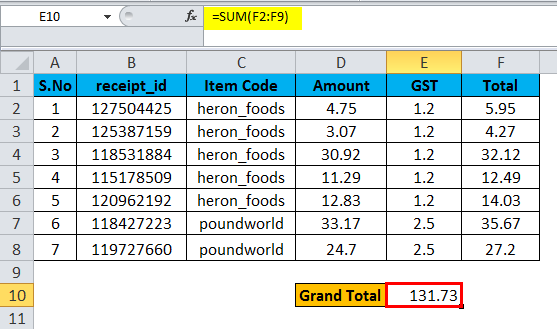
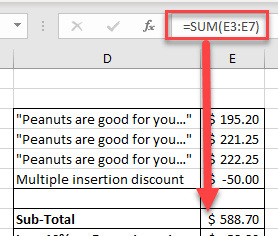
After applying the formula in the total column, the values are used to sum the Grand total. Now the formula bar is showing the current formula applied in cell E10. “=SUM (F2: F9)”, the range of cells is represented within the formula.
Formula Bar in Excel – Example #2
From the options available in the menu bar, it is possible to hide the formula bar as per your need. From the view menu, you can customize the tools you want to display in the available interface.
Go through the below steps to show or hide the formula bar within the excel sheet.
- Click on the View menu.
- Tick or untick the rectangle box given to enable or disable the formula bar.
- According to your selection, the visibility will be set.
How to Use Formula Bar Icons?
You can see some icons associated with the formula bar. It includes the icon next to the formula bar used for the following.
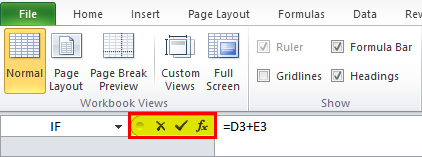
- × – This icon is to cancel edits and partial entry of the formula in the current cell.
- √ – Helps to edit the data in the current cell without moving the active highlighted cell to another.
- ƒx – This is a shortcut to insert the different functions used in the calculations.
The below dialogue box will drop down the different functions available.
The same can be activated using the shortcuts as
- Esc key – Remove the edits and a partial entry.
- Enter key – Edit the data in the current cell without moving the active highlighted cell to another.
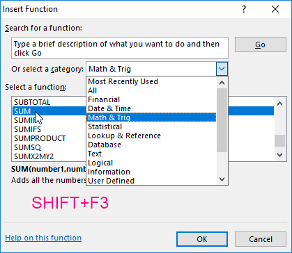
- Shift + F3 – To get the dialog box to insert the functions.
How to Expand the Visibility of Formula Bar?
By selecting the formula bar rather than the values, a formula will be displayed. While you are opening an excel sheet, the cells will show the values. But if you select a specific column, the formula applied to the cell will be shown in the formula bar.
If the formula bar is already expanded, then the “Collapse Formula Bar” option will be visible on the right click.
When you use complex formulas and many entries, the expansion of the formula bar is allowed. By expanding the formula bar, the data is wrapped into more than one line. This helps you to edit the formula easily other than doing it within the corresponding cell.
- By clicking the arrow at the end of the formula bar
- By expanding the mouse pointer selection with the two-headed arrow
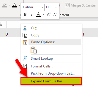
- By right-clicking, the formula bar select the option from the drop menu
The alternate option is to use the keyboard shortcut Ctrl + Shift + U. If the same keys are press repeatedly, then the default size will be restored.
To wrap the complex formulas or data into multiple lines, then point your selection where you want to break your data or formula, press Alt + Enter. The data or formula will be moved to the next line in the formula bar.
How to Protect the Formula from Unwanted Editing?
You can protect the formulas that you have applied in different cells. There are chances to delete the formulas when multiple persons are handling the same excel sheet. Using some simple steps, you can protect your formulas from editing by unauthorized users.
The first step is to hide the cells or range of cells where the formula being applied.
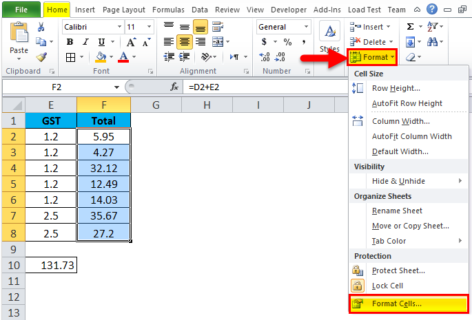
- Select the range of cells where you have already applied some formulas and want to hide. From the menu bar, click home and go to the format option to get a drop-down.
- Select the “Format Cells” option from the dropbox
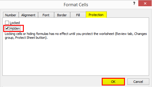
A dialog box will appear to select the “Protection” tab. Select the hidden checkbox by enabling the tick mark Press “OK” to apply your selection and close the dialog box.
The next stage is to enable the worksheet protection
- From the same format option given in the home menu, click for the drop-down.
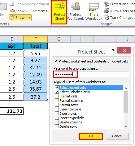
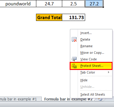
- Go to the “Protect Sheet” option from the drop-down list
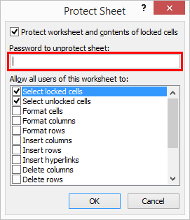
- You will get a dialogue box that helps you to give protection to the selected cells
- By checking the “Protect worksheet and contents of the locked cell”, the protection will be enabled
- For protecting the cells with the password, you have the option to give a password
- Once you want to unprotect the same selected cells, you can use the given password.
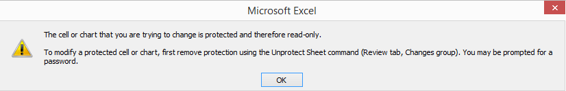
After setting the protection, if you try to make any changes, you will get a warning message to use the password to make any changes.
The same options are also available when you select the range of cells and right-click
While selecting the format cells, you will get the same dialog box to hide the formulas. To protect the sheet, you can right-click on the sheet name and will get the same dialog box to protect the sheet.
You will get a dialog box to set the password if you want to make the sheet password protected.
By using the shortcut key F2, it is possible to edit the active cell. This is a default setting if you need to make any change to this.
Go to the File menu in the “Option” menu will get Advanced editing options to disable the “Allow editing directly in the cell”.
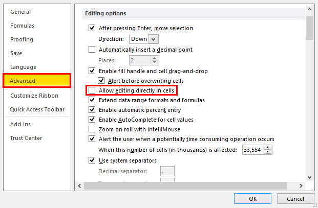
This will prevent unwanted editing of the inserted formula by mistake.
Things to Remember About Formula Bar in Excel
- Since the formula bar is always pointing to the active cell while applying the formula, you should ensure the active cell is correct.
- Better to use a formula bar for editing an applied formula. This will help you to manage the long formulas or data easily.
- Apart from the menu bar, use the shortcuts and right-click the selection to make your work easy.
- Ensure the formulas are protected from editing if you are sharing the excel document to multiple users. This will help to prevent data loss.
Recommended Articles
This is a guide to Formula Bar in Excel. Here we discuss how to use Formula Bar in Excel along with practical examples and a downloadable excel template. You can also go through our other suggested articles –
- How to Use Text Formula in Excel?
- Find and Replace in Excel
- Use of Freeze Columns in Excel
- Steps to Create Family Tree in Excel
The Formula Bar in Excel has more to it than what meets the eye and today’s tutorial will give you a rundown on it. (A run down and up if we’re honest!)
The Formula Bar is one of the core features of Excel and we will guide you on what it is, how to hide/display, expand/contract it, and how to use formula bar icons.
Let’s get formulating!

What is the Formula Bar in Excel
The Formula Bar in Excel shows the formula or value of a selected cell and can be used to edit any selected cell’s value. In the case of a formula, the cell will display the result while the Formula Bar will show the formula. The Formula Bar will display the underlying value of a cell while the cell may show a formatted value.
As soon as you start typing in a cell, the Formula Bar will start displaying the contents. The Formula Bar shows the contents of a single cell and therefore, in a selected range, the Formula Bar will show the contents of the first selected cell.
It is located between the column headers and the Ribbon, to the right of the Name Box. The given size of the Formula Bar is not a limitation, and it can be expanded or contracted vertically as well as horizontally. It is possible to completely hide and restore the Formula Bar.

How to Hide Formula Bar
By default, the Formula Bar is displayed in Excel. You might want to temporarily hide it to fit a few more rows into the worksheet space. Also, when you start typing in a cell, you are using the cell to add the contents instead of the Formula Bar so you might find that you prefer to hide the Formula Bar while working, making more rows visible too.
The Formula Bar can be hidden using the option in the View tab (by the mouse or keyboard) or in Excel Options. The methods are given below.
Method #1 – Using Ribbon Menu
Hide the Formula Bar in Excel by changing the view of the spreadsheet using the View tab in the Ribbon menu. The process is complete in a couple of clicks, here’s what to do:
- Go to the View tab in the Ribbon and click on the Formula Bar checkbox in the Show

- With the Formula Bar box unchecked, the Formula Bar has been removed from view:

After the Ribbon, the column headers have shifted upward, taking place of the Formula Bar. Check the Formula Bar box any time in the View tab to bring the Formula Bar back.
Method #2 – Using Excel Options
The next method of hiding the Formula Bar in Excel is through Excel Options. Find out how to access Options in Excel and how to use it to remove the Formula Bar from display with the steps given ahead:
- Select the File tab from the set of tabs above the Ribbon.
- Click on Options from the bottom of the left side pane.

- From the left panel, select the Advanced
- Scroll down to the Display section and unmark the Show formula bar

- Click on the OK button to apply the setting.
This will close the Excel Options dialog box, return you to the worksheet and hide the Formula Bar from display.

Method #3 – Using Keyboard Shortcut
Use the keyboard instead of the mouse to quickly remove the Formula Bar from view. This keyboard shortcut takes the route of the View tab to hide the Formula Bar. The keyboard shortcut for hiding the Formula Bar in Excel is:
Alt, W, V, F
Enter the keys above one after the other.
Alt key displays the shortcut keys for the tabs.
W key selects the View tab.
V, F keys select the Formula Bar checkbox.
The keyboard shortcut has led to the previously checked box being unchecked and therefore hiding the Formula Bar:

How to Show Formula Bar
If the Formula Bar has been hidden, using any one of the methods above will bring it back. While cells are mostly edited by direct typing, with the values of the surrounding cells, the contents of the active cell may become confusing, making the Formula Bar a better choice for editing data.
To restore the Formula Bar above the worksheet area, use one of the methods listed below.
Method #1 – Using Ribbon Menu
The Formula Bar option in the View tab is used to hide and unhide the Formula Bar in Excel. To unhide the Formula Bar:
- In the View tab’s Show group, check the Formula Bar box which should be unchecked at this point:

- After check-marking the box, the Formula Bar will be added back below the Ribbon:

Method #2 – Using Excel Options
To show the Formula Bar in the spreadsheet, you can use Excel Options. Follow these steps to bring the Formula Bar back on display:
- Select the File tab and then Options from the left.
- Next, select the Advanced tab and tick-mark the Show formula bar

- Hit the OK button to confirm the setting and close the dialog box.
The Formula Bar will return above the column headers:

Method #3 – Using Keyboard Shortcut
Use a keyboard shortcut to display the Formula Bar in Excel. This keyboard shortcut will lead to the View tab to select the Formula Bar checkbox. Enter the keys below in succession:
Alt, W, V, F
The Formula Bar box will be checked, showing the Formula Bar in the spreadsheet again:

How to Expand or Contract Formula Bar
The Formula Bar is not small by any means and can house a fairly long formula or cell value. But for longer formulas or cell values with line breaks, you will find that expanding the Formula Bar is much easier to work with. Also, when you’re working with multiple windows and have downsized your Excel window, the Formula Bar will consequently have lesser space than before.
The first suggestion to resize the Formula Bar is to resize your spreadsheet window. The drawback of that however is that a smaller window will not contract the Formula Bar to display the complete value of the cell or the formula; if either is too long, it will be hindered from view. Therefore, if it’s preferable not to resize the window, the Formula Bar can be contracted and expanded vertically in a couple of ways as well as horizontally. All three ways cater to resizing the Formula Bar differently. Details are given below.
Using Expand/Collapse Arrow
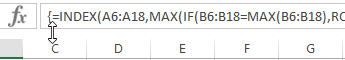
The small arrow at the end of the Formula Bar is for expanding or collapsing the Formula Bar. In the example ahead, the formula in cell E3 cannot be viewed completely. We will expand the Formula Bar to view the formula using the arrow:

The Formula Bar has expanded by another line and displays the whole formula now:

Note: This arrow will expand the Formula Bar to the size last set by the resizing arrow (coming up in the section ahead). If you haven’t used the resizing arrow before, the expanding arrow will only extend the Formula Bar by one more line.
Use the same arrow to contract the Formula Bar back to a single line:

Pro tip: Use the keyboard shortcut Ctrl + Shift + U to expand/collapse the Formula Bar. The shortcut toggles the Formula Bar‘s expand/collapse arrow.
Using Resizing Arrow
If the expand/collapse arrow isn’t giving you the right amount of view in the Formula Bar, you can expand the bar to the desired setting using the resizing arrow. You may be familiar with resizing arrows used on windows or objects. Two such arrows are available for the Formula Bar and they work to resize it vertically and horizontally (the latter explained in the next section).
This can be used as a preset for the expand/collapse arrow. We’ll let you know how. For now, have a look at the example case below. We have an address given in B13. The Formula Bar makes it evident that the address in B3 contains at least one line break as we cannot see the complete contents.
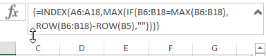
If we use the expand/collapse arrow at this point, we will only be able to view one more line and ideally, we should be able to view four in this case. To expand the Formula Bar to our preference, we will resize it instead by placing the cursor at the lower edge of the bar until a double-headed arrow appears:

Click and drag the Formula Bar using this arrow and extend it to the preferred length (four lines as per our example case). Now the Formula Bar will display the full contents of B13:

Use the same double-headed arrow to contract the Formula Bar to the preferred point or click the expand/collapse arrow once to restore the single-line Formula Bar.
After this, when you use the expand arrow, the Formula Bar will be extended to four lines instead of two since the expand arrow extends the Formula Bar to the last size set by the resizing arrow.
Resizing Horizontally
The Formula Bar in Excel can also be resized horizontally. You may need to expand the Formula Bar if you contracted it previously. Contracting it horizontally gives more room to the Name Box to display a longer name (e.g. of a range or cell).
Below in the example, we have named all the cells containing contact numbers as PhoneNumber, PhoneNumber2, and onwards so that they are easier to find. The Name Box with its current size can’t display the full name so we will resize the Formula Bar.
To contract the Formula Bar horizontally, place the cursor on the 3-dot menu icon between the Name Box and the formula bar icons until a double-headed arrow shows:

Click and drag to adjust the size of the Formula Bar. You can see below that the Formula Bar has contracted, expanding the Name Box:

Use the resizing arrow to expand the Formula Bar again or double-click the 3-dot menu to restore it to the default size.
Formula Bar Icons
The formula bar icons are used for actions regarding the Formula Bar. The icons are situated before the Formula Bar itself, on the right of the Name Box:

Now would be a good time to tell you what these icons represent and how they can be used. As a rule, the icons are usable if they change color from gray when you hover the cursor over them. If the icon remains gray, it is unusable at that time.
Cancel button – The Cancel button works as a replacement for the Esc key. It is only activated in cell edit mode i.e. the active cell (whether via the Formula Bar or the cell). Clicking on the button exits cell edit mode while the cell remains selected. If any changes have been made to the active cell, the Cancel button will revert the cell value to the value before editing, maintaining the cell selection. That means that the button only works for the edits of the active session.
Enter button – The Enter button works a bit like the Enter key but only for the active cell and also maintains the cell selection. If the button is used without making any changes to the active cell, cell edit mode will be exited while the cell remains selected. If the button is used after making changes to the active cell, the cell will take on the edited value, cell edit mode will be exited and the same cell will remain selected.
Insert Function button – The Insert Function button is used for inserting a function in a cell. It’s kind of like a functions encyclopedia. The button (or the Shift + F3 keys) opens the Insert Function dialog box where you can search for a function.

Search for a function by category. The default display of the functions is the Most Recently Used category. Other categories are groups of functions and can help you find a function according to those groups. The All category will alphabetically list all the functions.

Another easy way is to search for a function by entering a description. Functions with matching descriptions will be displayed for you to choose from. E.g., for counting blank cells, we can type the description «count blank cells» and hit Go. These would be the results:

The syntax and description of the selected function will be shown in the dialog box. (For more help, click on the Help on this function link at the bottom of the dialog box and it will lead to the Microsoft website.) Select a function by double-clicking it and you will be led to the Function Arguments dialog box which will aid you in forming the formula correctly with the arguments and will also break down the results:

When done, the OK button will enter the formula and display the results in the selected cell on the worksheet.
The Insert Function button does not need an active cell to be usable. In the active cell, it can only be used if the cell is either blank or contains a formula. With any other value present in the cell, the Insert Function button will remain disabled.
The button can be used on any selected cell (without entering cell edit mode). If the button is used on a cell containing a formula, the Function Arguments dialog box will open with the function that the blinking cursor is positioned on. Using this case as an example, if we keep the blinking cursor at the IF function in the formula, and select the Insert Function button,

The IF function will be emboldened in the Formula Bar while the Function Arguments dialog box opens with the details of the IF function in this particular formula:

Note that while Insert Function can overwrite a cell’s value, it cannot overwrite the format; the function used will result in the set cell format (if any).
Today we got up close and personal with the Formula Bar in Excel. Who should our next guest of honor be? We’ll get busy with that while you can experiment with the new bits and bobs you learned about the Formula Bar. Enough tricks we got there to keep you occupied? Only one way to find out. Ready? Tricky? Go!
Home / Excel Basics / Formula Bar in Excel
Written by Puneet for Excel 2007, Excel 2010, Excel 2013, Excel 2016, Excel 2019, Excel for Mac
Key Points
- You can hide and unhide the formula bar.
- You can change its height (expand it), but you can’t change its position.
What is the Excel Formula Bar?
Excel Formula Bar is a thin bar below the ribbon that displays the selected cell’s content and displays the cell address of the selected cell on the left side. You can also enter a value into the cell from the formula bar. It has three buttons (Enter, Cancel, and Insert a Function).


- Name Box
- Horizontal Expand
- Buttons
- Input bar
- Vertical Expand
How to Show Formula Bar (or Hide it)
The formula bar is active by default but if it is hidden, you can activate it from the view tab.
- First go to the view tab, and from the show group and tick mark formula bar.

- Apart from this, you can also activate it from the Excel options.
- Go to the Excel options ➜ Advanced ➜ Display ➜ Show formula bar.


You can use the same steps if you want to hide it.
Expand Formula Bar
By default, the formula bar is thin, but you can expand it and make it a little wide. When you hover your cursor on the bottom of the formula bar, it converts into a vertical double-ended arrow, and then you can pull it down to expand it.

There’s also a shortcut key (Control + Shift + U) that you can use to expand the formula bar vertically. You can also use the drop-down icon from the right side.

And if you want to change its width you can do it by hovering your cursor on the three dots between the name box and formula bar and then stretching it to the right or left.
[icon name=”bell” class=”” unprefixed_class=””] Excel Keyboard Shortcut Cheat Sheet
Enter Data from the Formula Bar
You can enter data into a cell by editing it from the formula bar, and for this, you need to select the cell and click on the input bar in the formula bar.

And once you are done with the value that you want to enter; you can click on the enter button that is on the left side of the formula bar.

There’s also a button to cancel the data entry or you can press the escape key.
Enter a Function using Formula Bar
There is an insert function button on the formula bar, and when you click on this button, it opens a dialogue box from which you can find and insert the function.

Once you select the function you want to insert, click OK, and it will show you a dialog box to define the function’s arguments.

Use Name Box
On the right side of the formula bar, you have a name box that shows the cell address for the selected cell. But you can also use this name box to navigate.
You are a specific cell or a range. When you click on the name box, it allows you to edit it, and you can enter a cell address, and once you do that and hit enter, it will navigate you to that cell.

In the same way, you can also enter a range’s address to select it.

Edit Shapes from Formula Bar
If you want to connect a shape with a cell, you can do that by editing it from the formula bar.

- Select the shape that you have in the worksheet.
- Click on the formula bar to edit it.
- Enter “=” and select the cell that you want to connect with the shape.
- In the end, click, OK.
See all How-To Articles
This tutorial explains the function of the formula bar in Excel and Google Sheets

The formula bar in Excel is above the column headers and below the Ribbon. The bar has the name box on the left, and the formula bar on the right.
Hide and Unhide the Formula Bar
If you cannot see the formula bar, it was probably hidden. There is an option in the Ribbon to show or hide the formula bar.
In the Ribbon, go to View > Show > Formula Bar.
Purpose of the Formula Bar
When you select a cell in a worksheet, the value in that cell shown in the formula bar either as a value/text or as a formula. You can use the formula bar to edit cells instead of typing directly into a cell.
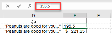
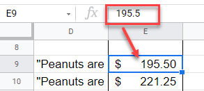
If you have formatted the data in your active cell (e.g., as a currency), then your worksheet displays the value in the cell as formatted. The formula bar, on the other hand, only shows the data in its “raw” data format without any formatting applied.
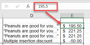
Similarly, if your cell contains a formula, the formula bar displays that formula, and the active cell displays the result.
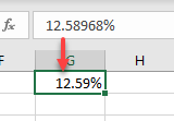
If a number has been formatted to have two decimal places but actually has a lot more (e.g., an interest rate), the formula bar shows all the decimal places, while the worksheet shows the number formatted to two decimal places.
View and Create Formulas
One of the most fundamental purposes of the formula bar is the ability to view and create formulas.
If you click on the cell that contains the formula, the formula shows up in the formula bar, while the result is shown in the active cell in the worksheet itself.
To create a formula, either type it into the cell, or enter directly into the formula bar.
Expand the Formula Bar
If you have a particularly long formula, you can expand the formula bar either horizontally or vertically.
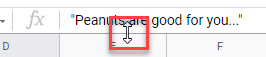
- To expand the formula bar vertically, move your mouse to the bottom of your formula bar until the cursor changes to a double-headed arrow.
![]()
- Click and drag the bottom of the formula bar down to increase its size.

If a single cell contains multiple lines of text, you can drag the formula bar down to show all the text in the cell.
- To expand the formula bar horizontally, move your mouse cursor between the name box and the formula bar. It changes to a double-headed arrow.
- Click and drag to the left to adjust the horizontal size of your formula bar.
You can also use the keyboard shortcut CTRL + SHIFT + U to expand and contract the formula bar. This adjusts it to a standard size or put it back to the default size.
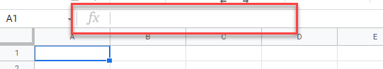
What is the Formula Bar in Google Sheets?
The formula bar in Google Sheets works very similarly.
As in Excel, the formula bar sits in the Google Sheet below the Menu and above the column headers.
You can view the raw data in the formula bar and the formatted data in the active cell in the sheet.
Or view the formula in the formula bar while seeing the result of that formula in the sheet.
You can edit the text or formula in the formula bar as well as directly in the sheet, and as in Excel, you can expand and contract the formula bar by placing your mouse at the bottom of the formula bar so your mouse pointer changes to a double-headed arrow, and dragging down until the formula bar is the right size.