
|
Вадим Озем  Пользователь Сообщений: 12 |
Не понимаю как вставить формулу через VBA для всего столбца Прикрепленные файлы
|
|
vikttur Пользователь Сообщений: 47199 |
Для всего столбца? Зачем Вам больше миллиона формул? |
|
Юрий М  Модератор Сообщений: 60588 Контакты см. в профиле |
Почему бы не вычислять макросом и вставлять не формулы, а сразу значения? |
|
МатросНаЗебре Пользователь Сообщений: 5516 |
#4 23.11.2021 12:44:59
|
||
|
Msi2102  Пользователь Сообщений: 3137 |
|
|
Вадим Озем Пользователь Сообщений: 12 |
Не для всего столбца, а пока в 1 столбце будет значение |
|
Юрий М Модератор Сообщений: 60588 Контакты см. в профиле |
#7 23.11.2021 13:48:27 Вадим Озем, перечитайте своё сообщение
Вам говорили не про количество столбцов, а про количество ячеек в столбце. |
||
|
bereteli  Пользователь Сообщений: 211 |
, можно маленький вопрос. Ваше сообщение означает расчет внутри vba? или подразумевается, что после просчета в экселе вставляются данные как значения? Изменено: bereteli — 23.11.2021 13:54:36 |
|
Вадим Озем Пользователь Сообщений: 12 |
#9 23.11.2021 13:55:35
Ну тут не столь важно, главное чтобы значение правильное было. |
||
|
vikttur Пользователь Сообщений: 47199 |
Тогда нужно предложить название темы, отражающее Вашу задачу. Что вычисляете? Предложите название. Заменят модераторы |
|
Юрий М Модератор Сообщений: 60588 Контакты см. в профиле |
#11 23.11.2021 14:06:15
Это мне адресовалось? Да, именно так. |
||
|
Вадим Озем Пользователь Сообщений: 12 |
Нужно расчет который будет в VBA и вставлять значения в ячейки в столбце C пока есть текст в ячейках столбца А |
|
_Igor_61  Пользователь Сообщений: 3007 |
#13 23.11.2021 14:46:02
На каком именно листе из двух листов в примере — пофиг |
||
|
Вадим Озем Пользователь Сообщений: 12 |
Формула которая в столбце C на листе Исходные данные должна считаться через VBA и вставить значение. А так же подвести итоги по столбцам D C B. желтым выделил где нужно формула в ячейках. А зеленым итоги Прикрепленные файлы
|
|
Msi2102 Пользователь Сообщений: 3137 |
Если правильно понял, то может так? Вставьте в столбец D формулу |
|
Вадим Озем Пользователь Сообщений: 12 |
Да вставить в столбец D формулу но через код макроса |
|
Msi2102 Пользователь Сообщений: 3137 |
Преобразуйте таблицу в УМНУЮ в первую ячейку столбца ИТОГ запишите формулу и эта формула будет проставлена во всём столбце, без макроса, также в умной таблице есть такое понятие, как Строка итогов |
|
Вадим Озем Пользователь Сообщений: 12 |
|
|
vikttur Пользователь Сообщений: 47199 |
|
|
МатросНаЗебре Пользователь Сообщений: 5516 |
#20 23.11.2021 16:55:07 И до кучи |
|
0 / 0 / 0 Регистрация: 18.10.2012 Сообщений: 28 |
|
|
1 |
|
|
10.11.2012, 13:34. Показов 14302. Ответов 15
Здравствуйте, по вопросам к VBA рекомендовали здешний форум. Вопрос первый: Второй вопрос: Заранее всем спасибо
0 |

|
Programming Эксперт 94731 / 64177 / 26122 Регистрация: 12.04.2006 Сообщений: 116,782 |
10.11.2012, 13:34 |
|
Ответы с готовыми решениями: Распространить зависимый список на весь столбец
15 |
") Нужно весь столбец скопировать, вставить в столбец A, так, чтобы вставились четырехзначные числа
Нужно весь столбец скопировать, вставить в столбец A, так, чтобы вставились четырехзначные числа|
Скрипт 5468 / 1148 / 50 Регистрация: 15.09.2012 Сообщений: 3,514 |
||||||||
|
10.11.2012, 14:39 |
2 |
|||||||
|
Вопрос первый:
Второй вопрос:
2 |
|
ST_Senya 0 / 0 / 0 Регистрация: 18.10.2012 Сообщений: 28 |
||||
|
11.11.2012, 10:11 [ТС] |
3 |
|||
|
Попробывал ваш код со списком, не получилось (см. рис), написал в коде кнопки
но на нужное мне место в списке так и не отобразилось, хотя если конечно самому вручную прокрутить полосу прокрутки, элемент выделен. Миниатюры
0 |

|
Скрипт 5468 / 1148 / 50 Регистрация: 15.09.2012 Сообщений: 3,514 |
||||||||
|
11.11.2012, 11:08 |
4 |
|||||||
|
ST_Senya, я неудачный дал пример кода. Вот попробуйте под себя это переделать:
List(20) — это содержимое 21 строки в ListBox (строки нумеруются в ListBox с нуля). Вот эта команда:
ищет в ListBox текст «1», если находит, то выделяет элемент, который содержит текст «1», и делает этот элемент видимым в ListBox, т.е. если есть полоса прокрутки, то поднимает ListBox так, чтобы было видно элемент, содержащий текст «1».
1 |
|
ST_Senya 0 / 0 / 0 Регистрация: 18.10.2012 Сообщений: 28 |
||||
|
11.11.2012, 14:19 [ТС] |
5 |
|||
|
Огромное спасибо, вот таким кодом всё получилось!
Теперь пользователь будет видеть какой файл обрабатывается в текущее время.
0 |
|
Скрипт 5468 / 1148 / 50 Регистрация: 15.09.2012 Сообщений: 3,514 |
||||
|
11.11.2012, 14:23 |
6 |
|||
|
CurrentSpisok — что это за элемент управления? У ListBox нет такого элемента ItemData.
0 |

|
0 / 0 / 0 Регистрация: 18.10.2012 Сообщений: 28 |
|
|
11.11.2012, 14:36 [ТС] |
7 |
|
У меня ACCESS 2007, элемент находится на форме (см рис. выше), называется список. Это графический элемент, где кнопки и др. элементы управления находятся. Я думал это и есть ListBox, значит он не так называется?
0 |
|
5468 / 1148 / 50 Регистрация: 15.09.2012 Сообщений: 3,514 |
|
|
11.11.2012, 14:46 |
8 |
|
ST_Senya,
под номером 1 название диалогового окна, где можно посмотреть класс элемента управления, под номером 2 — класс элемента управления.
0 |
|
0 / 0 / 0 Регистрация: 18.10.2012 Сообщений: 28 |
|
|
11.11.2012, 18:09 [ТС] |
9 |
|
Я его перетащил отсюда… Миниатюры
0 |
|
5468 / 1148 / 50 Регистрация: 15.09.2012 Сообщений: 3,514 |
|
|
11.11.2012, 18:17 |
10 |
|
ST_Senya, свойство Имя содержит название класса, когда элемент управления только создали. Какое имя даётся новому элементу управления, которое вы вставляете? У вас вообще не элементу управления, а элемент формы.
0 |
|
0 / 0 / 0 Регистрация: 18.10.2012 Сообщений: 28 |
|
|
11.11.2012, 18:22 [ТС] |
11 |
|
Тогда пардон…. Значит не так выразился. Значит элемент формы. В имени нет никакого класса. Да и бог с ним) Главное всё получилось. Возник следующий вопрос. Как мне отцентровать мои формы? а то когда я и открываю они открываются то слишком высоко, то слева где то. Как мне сделать что бы все они в зависимости от своих размеров располагались по центру экрана?
0 |
|
5468 / 1148 / 50 Регистрация: 15.09.2012 Сообщений: 3,514 |
|
|
11.11.2012, 18:24 |
12 |
|
ST_Senya, вы про Access 2007 ведёте речь?
0 |
|
0 / 0 / 0 Регистрация: 18.10.2012 Сообщений: 28 |
|
|
11.11.2012, 18:41 [ТС] |
13 |
|
У меня ACCESS 2007, элемент находится на форме (см рис. выше), называется список. Это графический элемент, где кнопки и др. элементы управления находятся. Я думал это и есть ListBox, значит он не так называется? Именно про него) Извините если ввожу в какие-то заблуждения. Дело в том что я создаю свою первую БД. И что в Аксессе, что в VBA не разбираюсь) только вот азы узнаю.
0 |
|
5468 / 1148 / 50 Регистрация: 15.09.2012 Сообщений: 3,514 |
|
|
11.11.2012, 18:43 |
14 |
|
ST_Senya, я про элементы Access не смогу помочь — с ним не работаю. Подождите, может кто другой поможет. Лучше создайте новую тему, потому что название этой темы никак не связана с Access.
0 |
|
0 / 0 / 0 Регистрация: 18.10.2012 Сообщений: 28 |
|
|
11.11.2012, 19:08 [ТС] |
15 |
|
Ну форма я думаю от Асесса не зависит. VBA он один думаю. Думаю что и форма Excel так же центруется
0 |
|
Скрипт 5468 / 1148 / 50 Регистрация: 15.09.2012 Сообщений: 3,514 |
||||
|
12.11.2012, 08:40 |
16 |
|||
|
ST_Senya, ListBox отличается, значит и ещё что-нибудь может отличаться. ST_Senya, по второму вопросу (сообщение #1) появилась новая информация. Чтобы отобразить выделенный элемент в ListBox, когда ListBox имеет полосу прокрутки, а выделенного элемента не видно, нужно использовать свойство TopIndex:
0 |
Вставка формулы со ссылками в стиле A1 и R1C1 в ячейку (диапазон) из кода VBA Excel. Свойства Range.FormulaLocal и Range.FormulaR1C1Local.
Свойство Range.FormulaLocal
FormulaLocal — это свойство объекта Range, которое возвращает или задает формулу на языке пользователя, используя ссылки в стиле A1.
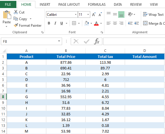
В качестве примера будем использовать диапазон A1:E10, заполненный числами, которые необходимо сложить построчно и результат отобразить в столбце F:

Примеры вставки формул суммирования в ячейку F1:
|
Range(«F1»).FormulaLocal = «=СУММ(A1:E1)» Range(«F1»).FormulaLocal = «=СУММ(A1;B1;C1;D1;E1)» |
Пример вставки формул суммирования со ссылками в стиле A1 в диапазон F1:F10:
|
Sub Primer1() Dim i As Byte For i = 1 To 10 Range(«F» & i).FormulaLocal = «=СУММ(A» & i & «:E» & i & «)» Next End Sub |
В этой статье я не рассматриваю свойство Range.Formula, но если вы решите его применить для вставки формулы в ячейку, используйте англоязычные функции, а в качестве разделителей аргументов — запятые (,) вместо точек с запятой (;):
|
Range(«F1»).Formula = «=SUM(A1,B1,C1,D1,E1)» |
После вставки формула автоматически преобразуется в локальную (на языке пользователя).
Свойство Range.FormulaR1C1Local
FormulaR1C1Local — это свойство объекта Range, которое возвращает или задает формулу на языке пользователя, используя ссылки в стиле R1C1.
Формулы со ссылками в стиле R1C1 можно вставлять в ячейки рабочей книги Excel, в которой по умолчанию установлены ссылки в стиле A1. Вставленные ссылки в стиле R1C1 будут автоматически преобразованы в ссылки в стиле A1.
Примеры вставки формул суммирования со ссылками в стиле R1C1 в ячейку F1 (для той же таблицы):
|
‘Абсолютные ссылки в стиле R1C1: Range(«F1»).FormulaR1C1Local = «=СУММ(R1C1:R1C5)» Range(«F1»).FormulaR1C1Local = «=СУММ(R1C1;R1C2;R1C3;R1C4;R1C5)» ‘Ссылки в стиле R1C1, абсолютные по столбцам и относительные по строкам: Range(«F1»).FormulaR1C1Local = «=СУММ(RC1:RC5)» Range(«F1»).FormulaR1C1Local = «=СУММ(RC1;RC2;RC3;RC4;RC5)» ‘Относительные ссылки в стиле R1C1: Range(«F1»).FormulaR1C1Local = «=СУММ(RC[-5]:RC[-1])» Range(«F2»).FormulaR1C1Local = «=СУММ(RC[-5];RC[-4];RC[-3];RC[-2];RC[-1])» |
Пример вставки формул суммирования со ссылками в стиле R1C1 в диапазон F1:F10:
|
‘Ссылки в стиле R1C1, абсолютные по столбцам и относительные по строкам: Range(«F1:F10»).FormulaR1C1Local = «=СУММ(RC1:RC5)» ‘Относительные ссылки в стиле R1C1: Range(«F1:F10»).FormulaR1C1Local = «=СУММ(RC[-5]:RC[-1])» |
Так как формулы с относительными ссылками и относительными по строкам ссылками в стиле R1C1 для всех ячеек столбца F одинаковы, их можно вставить сразу, без использования цикла, во весь диапазон.
In this lesson you can learn how to add a formula to a cell using vba. There are several ways to insert formulas to cells automatically. We can use properties like Formula, Value and FormulaR1C1 of the Range object. This post explains five different ways to add formulas to cells.
Table of contents
How to add formula to cell using VBA
Add formula to cell and fill down using VBA
Add sum formula to cell using VBA
How to add If formula to cell using VBA
Add formula to cell with quotes using VBA
Add Vlookup formula to cell using VBA
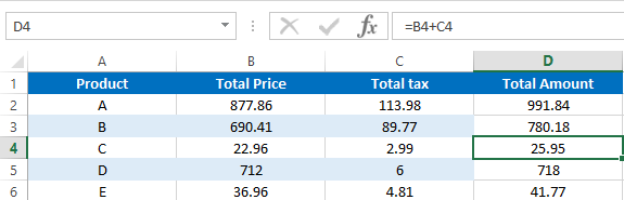
We use formulas to calculate various things in Excel. Sometimes you may need to enter the same formula to hundreds or thousands of rows or columns only changing the row numbers or columns. For an example let’s consider this sample Excel sheet.
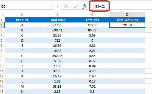
In this Excel sheet I have added a very simple formula to the D2 cell.
=B2+C2
So what if we want to add similar formulas for all the rows in column D. So the D3 cell will have the formula as =B3+C3 and D4 will have the formula as =B4+D4 and so on. Luckily we don’t need to type the formulas manually in all rows. There is a much easier way to do this. First select the cell containing the formula. Then take the cursor to the bottom right corner of the cell. Mouse pointer will change to a + sign. Then left click and drag the mouse until the end of the rows.
However if you want to add the same formula again and again for lots of Excel sheets then you can use a VBA macro to speed up the process. First let’s look at how to add a formula to one cell using vba.
How to add formula to cell using VBA
Lets see how we can enter above simple formula(=B2+C2) to cell D2 using VBA
In this method we are going to use the Formula property of the Range object.
Sub AddFormula_Method1()
Dim WS As Worksheet
Set WS = Worksheets(«Sheet1»)
WS.Range(«D2»).Formula = «=B2+C2»
End Sub
We can also use the Value property of the Range object to add a formula to a cell.
Sub AddFormula_Method2()
Dim WS As Worksheet
Set WS = Worksheets(«Sheet1»)
WS.Range(«D2»).Value = «=B2+C2»
End Sub
Next method is to use the FormulaR1C1 property of the Range object. There are few different ways to use FormulaR1C1 property. We can use absolute reference, relative reference or use both types of references inside the same formula.
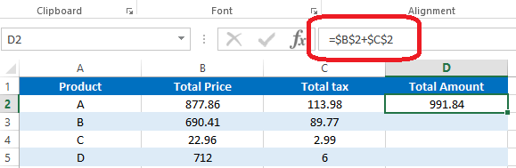
In the absolute reference method cells are referred to using numbers. Excel sheets have numbers for each row. So you should think similarly for columns. So column A is number 1. Column B is number 2 etc. Then when writing the formula use R before the row number and C before the column number. So the cell A1 is referred to by R1C1. A2 is referred to by R2C1. B3 is referred to by R3C2 etc.
This is how you can use the absolute reference.
Sub AddFormula_Method3A()
Dim WS As Worksheet
Set WS = Worksheets(«Sheet1»)
WS.Range(«D2»).FormulaR1C1 = «=R2C2+R2C3»
End Sub
If you use the absolute reference, the formula will be added like this.
If you use the manual drag method explained above to fill down other rows, then the same formula will be copied to all the rows.
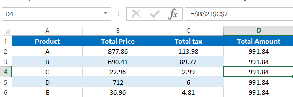
In Majority cases this is not how you want to fill down the formula. However this won’t happen in the relative method. In the relative method, cells are given numbers relative to the cell where the formula is entered. You should use negative numbers when referring to the cells in upward direction or left. Also the numbers should be placed within the square brackets. And you can omit [0] when referring to cells on the same row or column. So you can use RC[-2] instead of R[0]C[-2]. The macro recorder also generates relative reference type code, if you enter a formula to a cell while enabling the macro recorder.
Below example shows how to put formula =B2+C2 in D2 cell using relative reference method.
Sub AddFormula_Method3B()
Dim WS As Worksheet
Set WS = Worksheets(«Sheet1»)
WS.Range(«D2»).FormulaR1C1 = «=RC[-2]+RC[-1]»
End Sub
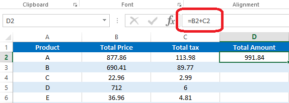
Now use the drag method to fill down all the rows.
You can see that the formulas are changed according to the row numbers.
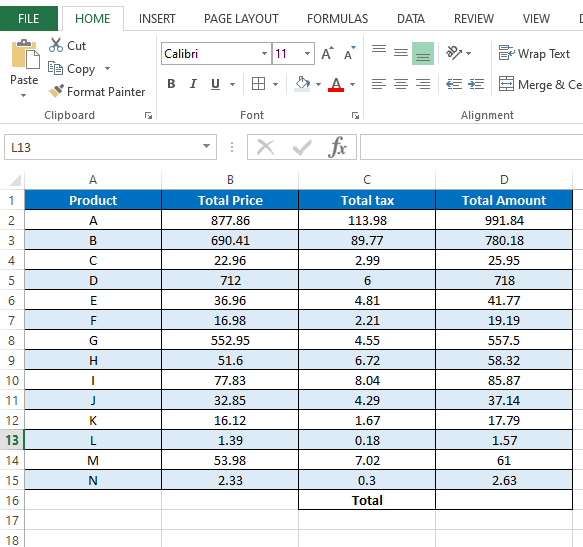
Also you can use both relative and absolute references in the same formula. Here is a typical example where you need a formula with both reference types.
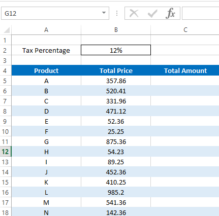
We can add the formula to calculate Total Amount like this.
Sub AddFormula_Method3C()
Dim WS As Worksheet
Set WS = Worksheets(«Sheet2»)
WS.Range(«C5»).FormulaR1C1 = «=RC[-1]+RC[-1]*R2C2»
End Sub
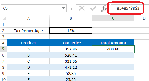
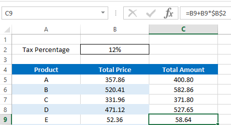
In this formula we have a absolute reference after the * symbol. So when we fill down the formula using the drag method that part will remain the same for all the rows. Hence we will get correct results for all the rows.
Add formula to cell and fill down using VBA
So now you’ve learnt various methods to add a formula to a cell. Next let’s look at how to fill down the other rows with the added formula using VBA.
Assume we have to calculate cell D2 value using =B2+C2 formula and fill down up to 1000 rows. First let’s see how we can modify the first method to do this. Let’s name this subroutine as “AddFormula_Method1_1000Rows”
Sub AddFormula_Method1_1000Rows()
End Sub
Then we need an additional variable for the For Next statement
Dim WS As Worksheet
Dim i As Integer
Next, assign the worksheet to WS variable
Set WS = Worksheets(«Sheet1»)
Now we can add the For Next statement like this.
For i = 2 To 1000
WS.Range(«D» & i).Formula = «=B» & i & «+C» & i
Next i
Here I have used «D» & i instead of D2 and «=B» & i & «+C» & i instead of «=B2+C2». So the formula keeps changing like =B3+C3, =B4+C4, =B5+C5 etc. when iterated through the For Next loop.
Below is the full code of the subroutine.
Sub AddFormula_Method1_1000Rows()
Dim WS As Worksheet
Dim i As Integer
Set WS = Worksheets(«Sheet1»)
For i = 2 To 1000
WS.Range(«D» & i).Formula = «=B» & i & «+C» & i
Next i
End Sub
So that’s how you can use VBA to add formulas to cells with variables.
Next example shows how to modify the absolute reference type of FormulaR1C1 method to add formulas upto 1000 rows.
Sub AddFormula_Method3A_1000Rows()
Dim WS As Worksheet
Dim i As Integer
Set WS = Worksheets(«Sheet1»)
For i = 2 To 1000
WS.Range(«D» & i).FormulaR1C1 = «=R» & i & «C2+R» & i & «C3»
Next i
End Sub
You don’t need to do any change to the formula section when modifying the relative reference type of the FormulaR1C1 method.
Sub AddFormula_Method3B_1000Rows()
Dim WS As Worksheet
Dim i As Integer
Set WS = Worksheets(«Sheet1»)
For i = 2 To 1000
WS.Range(«D» & i).FormulaR1C1 = «=RC[-2]+RC[-1]»
Next i
End Sub
Use similar techniques to modify other two types of subroutines to add formulas for multiple rows. Now you know how to add formulas to cells with a variable. Next let’s look at how to add formulas with some inbuilt functions using VBA.
How to add sum formula to a cell using VBA
Suppose we want the total of column D in the D16 cell. So this is the formula we need to create.
=SUM(D2:D15)
Now let’s see how to add this using VBA. Let’s name this subroutine as SumFormula.
First let’s declare a few variables.
Dim WS As Worksheet
Dim StartingRow As Long
Dim EndingRow As Long
Assign the worksheet to the variable.
Set WS = Worksheets(«Sheet3»)
Assign the starting row and the ending row to relevant variables.
StartingRow = 2
EndingRow = 1
Then the final step is to create the formula with the above variables.
WS.Range(«D16»).Formula = «=SUM(D» & StartingRow & «:D» & EndingRow & «)»
Below is the full code to add the Sum formula using VBA.
Sub SumFormula()
Dim WS As Worksheet
Dim StartingRow As Long
Dim EndingRow As Long
Set WS = Worksheets(«Sheet3»)
StartingRow = 2
EndingRow = 15
WS.Range(«D16»).Formula = «=SUM(D» & StartingRow & «:D» & EndingRow & «)»
End Sub
How to add If Formula to a cell using VBA
If function is a very popular inbuilt worksheet function available in Microsoft Excel. This function has 3 arguments. Two of them are optional.
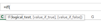
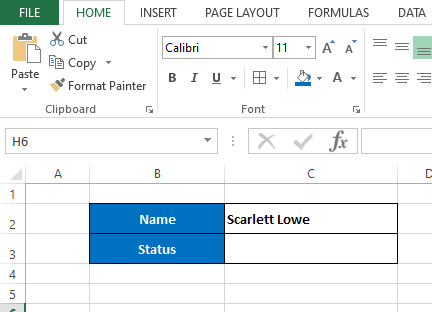
Now let’s see how to add a If formula to a cell using VBA. Here is a typical example where we need a simple If function.
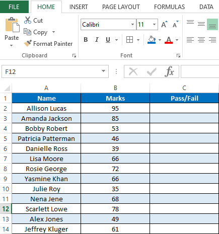
This is the results of students on an examination. Here we have names of students in column A and their marks in column B. Students should get “Pass” if he/she has marks equal or higher than 40. If marks are less than 40 then Excel should show the “Fail” in column C. We can simply obtain this result by adding an If function to column C. Below is the function we need in the C2 cell.
=IF(B2>=40,»Pass»,»Fail»)
Now let’s look at how to add this If Formula to a C2 cell using VBA. Once you know how to add it then you can use the For Next statement to fill the rest of the rows like we did above. We discussed a few different ways to add formulas to a range object using VBA. For this particular example I’m going to use the Formula property of the Range object.
So now let’s see how we can develop this macro. Let’s name this subroutine as “AddIfFormula”
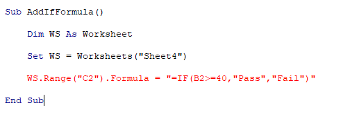
Sub AddIfFormula()
End Sub
However we can’t simply add this If formula using the Formula property like we did before. Because this If formula has quotes inside it. So if we try to add the formula to the cell with quotes, then we get a syntax error.
Add formula to cell with quotes
There are two ways to add the formula to a cell with quotes.
Sub AddIfFormula_Method1()
Dim WS As Worksheet
Set WS = Worksheets(«Sheet4»)
WS.Range(«C2»).Formula = «=IF(B2>=40,»»Pass»»,»»Fail»»)»
End Sub
Sub AddIfFormula_Method2()
Dim WS As Worksheet
Set WS = Worksheets(«Sheet4»)
WS.Range(«C2»).Formula = «=IF(B2>=40,» & Chr(34) & «Pass» & Chr(34) & «,» & Chr(34) & «Fail» & Chr(34) & «)»
End Sub
Add vlookup formula to cell using VBA
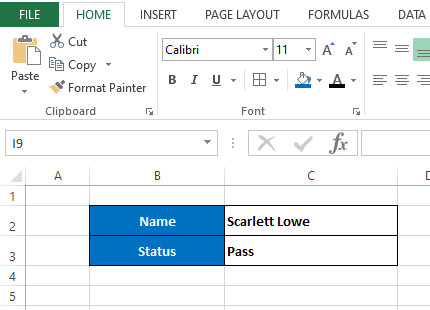
Finally I will show you how to add a vlookup formula to a cell using VBA. So I created a very simple example where we can use a Vlookup function. Assume we have this section in the Sheet5 of the same workbook.
So here when we change the name of the student in the C2 cell, his/her pass or fail status should automatically be shown in the C3 cell. If the original data(data we used in the above “If formula” example) is listed in the Sheet4 then we can write a Vlookup formula for the C3 cell like this.
=VLOOKUP(Sheet5!C2,Sheet4!A2:C200,3,FALSE)
We can use the Formula property of the Range object to add this Vlookup formula to the C3 using VBA.
Sub AddVlookupFormula()
Dim WS As Worksheet
Set WS = Worksheets(«Sheet5»)
WS.Range(«C3»).Formula = «=VLOOKUP(Sheet5!C2,Sheet4!A2:C200,3,FALSE)»
End Sub
In Excel, you can use VBA to calculate the sum of values from a range of cells or multiple ranges. And, in this tutorial, we are going to learn the different ways that we can use this.
Sum in VBA using WorksheetFunction
In VBA, there are multiple functions that you can use, but there’s no specific function for this purpose. That does not mean we can’t do a sum. In VBA, there’s a property called WorksheetFunction that can help you to call functions into a VBA code.

Let sum values from the range A1:A10.
- First, enter the worksheet function property and then select the SUM function from the list.

- Next, you need to enter starting parenthesis as you do while entering a function in the worksheet.

- After that, we need to use the range object to refer to the range for which we want to calculate the sum.

- In the end, type closing parenthesis and assign the function’s returning value to cell B1.


Range("B1") = Application.WorksheetFunction.Sum(Range("A1:A10"))Now when you run this code, it will calculate the sum for the values that you have in the range A1:A10 and enter the value in cell B1.

Sum Values from an Entire Column or a Row
In that just need to specify a row or column instead of the range that we have used in the earlier example.
'for the entire column A
Range("B1") = Application.WorksheetFunction.Sum(Range("A:A"))

'for entire row 1
Range("B1") = Application.WorksheetFunction.Sum(Range("1:1"))
Use VBA to Sum Values from the Selection
Now let’s say you want to sum value from the selected cells only in that you can use a code just like the following.
Sub vba_sum_selection()

Dim sRange As Range
Dim iSum As Long

On Error GoTo errorHandler

Set sRange = Selection

iSum = WorksheetFunction.Sum(Range(sRange.Address))
MsgBox iSum

errorHandler:
MsgBox "make sure to select a valid range of cells"

End Sub
In the above code, we have used the selection and then specified it to the variable “sRange” and then use that range variable’s address to get the sum.
The following code takes all the cells and sum values from them and enters the result in the selected cell.
Sub vba_auto_sum()

Dim iFirst As String
Dim iLast As String
Dim iRange As Range

On Error GoTo errorHandler

iFirst = Selection.End(xlUp).End(xlUp).Address
iLast = Selection.End(xlUp).Address

Set iRange = Range(iFirst & ":" & iLast)
ActiveCell = WorksheetFunction.Sum(iRange)

Exit Sub

errorHandler:
MsgBox "make sure to select a valid range of cells"

End Sub
Sum a Dynamic Range using VBA
And in the same way, you can use a dynamic range while using VBA to sum values.
Sub vba_dynamic_range_sum()

Dim iFirst As String
Dim iLast As String
Dim iRange As Range

On Error GoTo errorHandler

iFirst = Selection.Offset(1, 1).Address
iLast = Selection.Offset(5, 5).Address

Set iRange = Range(iFirst & ":" & iLast)
ActiveCell = WorksheetFunction.Sum(iRange)

Exit Sub

errorHandler:
MsgBox "make sure to select a valid range of cells"

End Sub
Sum a Dynamic Column or a Row
In the same way, if you want to use a dynamic column you can use the following code where it will take the column of the active cell and sum for all the values that you have in it.
Sub vba_dynamic_column()

Dim iCol As Long

On Error GoTo errorHandler

iCol = ActiveCell.Column
MsgBox WorksheetFunction.Sum(Columns(iCol))

Exit Sub

errorHandler:
MsgBox "make sure to select a valid range of cells"

End Sub
And for a row.
Sub vba_dynamic_row()

Dim iRow As Long

On Error GoTo errorHandler

iRow = ActiveCell.Row

MsgBox WorksheetFunction.Sum(Rows(iCol))

Exit Sub

errorHandler:
MsgBox "make sure to select a valid range of cells"

End Sub
Using SUMIF with VBA
Just like sum you can use the SUMIF function to sum values with criteria just like the following example.

Sub vba_sumif()

Dim cRange As Range
Dim sRange As Range

Set cRange = Range("A2:A13")
Set sRange = Range("B2:B13")

Range("C2") = _
WorksheetFunction.SumIf(cRange, "Product B", sRange)

End Sub