
Содержание
- Format text in cells
- Change font style, size, color, or apply effects
- Change the text alignment
- Clear formatting
- Change font style, size, color, or apply effects
- Change the text alignment
- Clear formatting
- How to control and understand settings in the Format Cells dialog box in Excel
- Summary
- More Information
- Number Tab
- Auto Number Formatting
- Built-in Number Formats
- Custom Number Formats
- Change the display of chart axes
- Learn more about axes
- Display or hide axes
- Adjust axis tick marks and labels
- Change the number of categories between labels or tick marks
- Change the alignment and orientation of labels
- Change text of category labels
- Change how text and numbers look in labels
- Change the display of chart axes in Office 2010
- Add tick marks on an axis
- All about axes
Format text in cells
Formatting text or numbers can make them appear more visible especially when you have a large worksheet. Changing default formats includes things like changing the font color, style, size, text alignment in a cell, or apply formatting effects. This article shows you how you can apply different formats and also undo them.
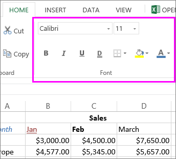
If you want text or numbers in a cell to appear bold, italic, or have a single or double underline, select the cell and on the Home tab, pick the format you want:
Change font style, size, color, or apply effects
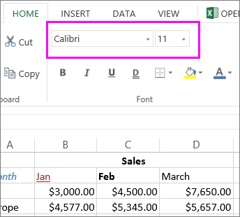
For a different font style, click the arrow next to the default font Calibri and pick the style you want.
To increase or decrease the font size, click the arrow next to the default size 11 and pick another text size.
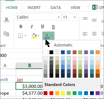
To change the font color, click Font Color and pick a color.
To add a background color, click Fill Color next to Font Color .
To apply strikethrough, superscript, or subscript formatting, click the Dialog Box Launcher, and select an option under Effects.
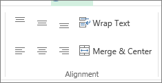
Change the text alignment
You can position the text within a cell so that it is centered, aligned left or right. If it’s a long line of text, you can apply Wrap Text so that all the text is visible.
Select the text that you want to align, and on the Home tab, pick the alignment option you want.
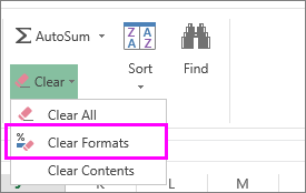
Clear formatting
If you change your mind after applying any formatting, to undo it, select the text, and on the Home tab, click Clear > Clear Formats.
Change font style, size, color, or apply effects
For a different font style, click the arrow next to the default font Calibri and pick the style you want.
To increase or decrease the font size, click the arrow next to the default size 11 and pick another text size.
To change the font color, click Font Color and pick a color.
To add a background color, click Fill Color next to Font Color .
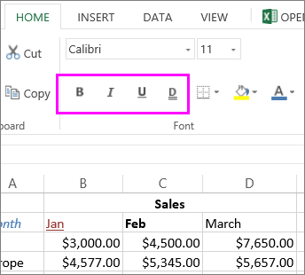
For boldface, italics, underline, double underline, and strikethrough, select the appropriate option under Font.

Change the text alignment
You can position the text within a cell so that it is centered, aligned left or right. If it’s a long line of text, you can apply Wrap Text so that all the text is visible.
Select the text that you want to align, and on the Home tab, pick the alignment option you want.
Clear formatting
If you change your mind after applying any formatting, to undo it, select the text, and on the Home tab, click Clear > Clear Formats.
Источник
How to control and understand settings in the Format Cells dialog box in Excel
Summary
Microsoft Excel lets you change many of the ways it displays data in a cell. For example, you can specify the number of digits to the right of a decimal point, or you can add a pattern and border to the cell. You can access and modify the majority of these settings in the Format Cells dialog box (on the Format menu, click Cells).
The «More Information» section of this article provides information about each of the settings available in the Format Cells dialog box and how each of these settings can affect the way your data is presented.
More Information
There are six tabs in the Format Cells dialog box: Number, Alignment, Font, Border, Patterns, and Protection. The following sections describe the settings available in each tab.
Number Tab
Auto Number Formatting
By default, all worksheet cells are formatted with the General number format. With the General format, anything you type into the cell is usually left as-is. For example, if you type 36526 into a cell and then press ENTER, the cell contents are displayed as 36526. This is because the cell remains in the General number format. However, if you first format the cell as a date (for example, d/d/yyyy) and then type the number 36526, the cell displays 1/1/2000.
There are also other situations where Excel leaves the number format as General, but the cell contents are not displayed exactly as they were typed. For example, if you have a narrow column and you type a long string of digits like 123456789, the cell might instead display something like 1.2E+08. If you check the number format in this situation, it remains as General.
Finally, there are scenarios where Excel may automatically change the number format from General to something else, based on the characters that you typed into the cell. This feature saves you from having to manually make the easily recognized number format changes. The following table outlines a few examples where this can occur:
| If you type | Excel automatically assigns this number format |
|---|---|
| 1.0 | General |
| 1.123 | General |
| 1.1% | 0.00% |
| 1.1E+2 | 0.00E+00 |
| 1 1/2 | # ?/? |
| $1.11 | Currency, 2 decimal places |
| 1/1/01 | Date |
| 1:10 | Time |
Generally speaking, Excel applies automatic number formatting whenever you type the following types of data into a cell:
Built-in Number Formats
Excel has a large array of built-in number formats from which you can choose. To use one of these formats, click any one of the categories below General and then select the option that you want for that format. When you select a format from the list, Excel automatically displays an example of the output in the Sample box on the Number tab. For example, if you type 1.23 in the cell and you select Number in the category list, with three decimal places, the number 1.230 is displayed in the cell.
These built-in number formats actually use a predefined combination of the symbols listed below in the «Custom Number Formats» section. However, the underlying custom number format is transparent to you.
The following table lists all of the available built-in number formats:
| Number format | Notes |
|---|---|
| Number | Options include: the number of decimal places, whether or not the thousands separator is used, and the format to be used for negative numbers. |
| Currency | Options include: the number of decimal places, the symbol used for the currency, and the format to be used for negative numbers. This format is used for general monetary values. |
| Accounting | Options include: the number of decimal places, and the symbol used for the currency. This format lines up the currency symbols and decimal points in a column of data. |
| Date | Select the style of the date from the Type list box. |
| Time | Select the style of the time from the Type list box. |
| Percentage | Multiplies the existing cell value by 100 and displays the result with a percent symbol. If you format the cell first and then type the number, only numbers between 0 and 1 are multiplied by 100. The only option is the number of decimal places. |
| Fraction | Select the style of the fraction from the Type list box. If you do not format the cell as a fraction before typing the value, you may have to type a zero or space before the fractional part. For example, if the cell is formatted as General and you type 1/4 in the cell, Excel treats this as a date. To type it as a fraction, type 0 1/4 in the cell. |
| Scientific | The only option is the number of decimal places. |
| Text | Cells formatted as text will treat anything typed into the cell as text, including numbers. |
| Special | Select one of the following from the Type box: Zip Code, Zip Code + 4, Phone Number, and Social Security Number. |
Custom Number Formats
If one of the built-in number formats does not display the data in the format that you require, you can create your own custom number format. You can create these custom number formats by modifying the built-in formats or by combining the formatting symbols into your own combination.
Before you create your own custom number format, you need to be aware of a few simple rules governing the syntax for number formats:
Each format that you create can have up to three sections for numbers and a fourth section for text.
The first section is the format for positive numbers, the second for negative numbers, and the third for zero values.
These sections are separated by semicolons.
If you have only one section, all numbers (positive, negative, and zero) are formatted with that format.
You can prevent any of the number types (positive, negative, zero) from being displayed by not typing symbols in the corresponding section. For example, the following number format prevents any negative or zero values from being displayed:
To set the color for any section in the custom format, type the name of the color in brackets in the section. For example, the following number format formats positive numbers blue and negative numbers red:
Instead of the default positive, negative and zero sections in the format, you can specify custom criteria that must be met for each section. The conditional statements that you specify must be contained within brackets. For example, the following number format formats all numbers greater than 100 as green, all numbers less than or equal to -100 as yellow, and all other numbers as cyan:
Источник
Change the display of chart axes
For most chart types, you can display or hide chart axes. To make chart data easier to understand, you can also change the way they look.
Important: This article does NOT cover changing the scale of chart axes. For information about how to change to the scale, see:
Learn more about axes
Charts typically have two axes that are used to measure and categorize data: a vertical axis (also known as value axis or y axis), and a horizontal axis (also known as category axis or x axis). 3-D column, 3-D cone, or 3-D pyramid charts have a third axis, the depth axis (also known as series axis or z axis), so that data can be plotted along the depth of a chart. Radar charts do not have horizontal (category) axes, and pie and doughnut charts do not have any axes.
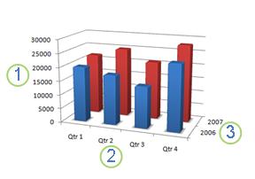
 Vertical (value) axis
 Horizontal (category) axis
 Depth (series) axis
The following describe how you can modify your charts to add impact and better convey information. For more info on what axes are and what you can do with them, see All about axes.
Note: The following procedure applies to Office 2013 and newer versions. Looking for Office 2010 steps?
Display or hide axes
Click anywhere in the chart for which you want to display or hide axes.
This displays the Chart Tools, adding the Design, and Format tabs.
On the Design tab, click the down arrow next to Add chart elements, and then hover over Axes in the fly-out menu .
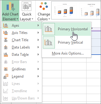
Click the type of axis that you want to display or hide.
Adjust axis tick marks and labels
On a chart, click the axis that has the tick marks and labels that you want to adjust, or do the following to select the axis from a list of chart elements:
Click anywhere in the chart.
This displays the Chart Tools, adding the Design and Format tabs.
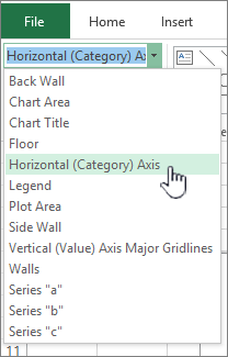
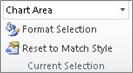
On the Format tab, in the Current Selection group, click the arrow in the Chart Elements box, and then click the axis that you want to select.
On the Format tab, in the Current Selection group, click Format Selection.
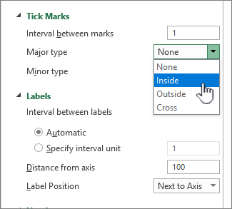
In the Axis Options panel, under Tick Marks, do one or more of the following:
To change the display of major tick marks, in the Major tick mark type box, click the tick mark position that you want.
To change the display of minor tick marks, in the Minor tick mark type drop-down list box, click the tick mark position that you want.
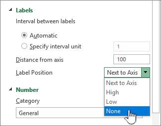
To change the position of the labels, under Labels, click the option that you want.
Tip To hide tick marks or tick-mark labels, in the Axis labels box, click None.
Change the number of categories between labels or tick marks
On a chart, click the horizontal (category) axis that you want to change, or do the following to select the axis from a list of chart elements:
Click anywhere in the chart.
This displays the Chart Tools, adding the Design, Layout, and Format tabs.
On the Format tab, in the Current Selection group, click the arrow in the Chart Elements box, and then click the axis that you want to select.
On the Format tab, in the Current Selection group, click Format Selection.
Under Axis Options, do one or both of the following:
To change the interval between axis labels, under Interval between labels, click Specify interval unit, and then in the text box, type the number that you want.
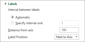
Tip Type 1 to display a label for every category, 2 to display a label for every other category, 3 to display a label for every third category, and so on.
To change the placement of axis labels, in the Label distance from axis box, type the number that you want.
Tip Type a smaller number to place the labels closer to the axis. Type a larger number if you want more distance between the label and the axis.
Change the alignment and orientation of labels
You can change the alignment of axis labels on both horizontal (category) and vertical (value) axes. When you have multiple-level category labels in your chart, you can change the alignment of all levels of labels. You can also change the amount of space between levels of labels on the horizontal (category) axis.
On a chart, click the axis that has the labels that you want to align differently, or do the following to select the axis from a list of chart elements:
Click anywhere in the chart.
This displays the Chart Tools, adding the Design and Format tabs.
On the Format tab, in the Current Selection group, click the arrow in the Chart Elements box, and then click the axis that you want to select.
On the Format tab, in the Current Selection group, click Format Selection.
In the Format Axis dialog box, click Text Options.
Under Text Box, do one or more of the following:
In the Vertical alignment box, click the vertical alignment position that you want.
In the Text direction box, click the text orientation that you want.
In the Custom angle box, select the degree of rotation that you want.
Tip You can also change the horizontal alignment of axis labels, by clicking the axis, and then click Align Left  , Center
  , or Align Right
  on the Home toolbar.
Change text of category labels
You can change the text of category labels on the worksheet, or you can change them directly in the chart.
Change category label text on the worksheet
On the worksheet, click the cell that contains the name of the label that you want to change.
Type the new name, and then press ENTER.
Note Changes that you make on the worksheet are automatically updated in the chart.
Change the label text in the chart
In the chart, click the horizontal axis, or do the following to select the axis from a list of chart elements:
Click anywhere in the chart.
This displays the Chart Tools, adding the Design and Format tabs.
On the Format tab, in the Current Selection group, click the arrow in the Chart Elements box, and then click the horizontal (category) axis.
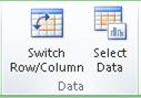
On the Design tab, in the Data group, click Select Data.
In the Select Data Source dialog box, under Horizontal (Categories) Axis Labels, click Edit.
In the Axis label range box, do one of the following:
Specify the worksheet range that you want to use as category axis labels.
Type the labels that you want to use, separated by commas — for example, Division A, Division B, Division C.
Note If you type the label text in the Axis label range box, the category axis label text is no longer linked to a worksheet cell.
Change how text and numbers look in labels
You can change the format of text in category axis labels or numbers on the value axis.
In a chart, right-click the axis that displays the labels that you want to format.
On the Home toolbar, click the formatting options that you want.
Tip You can also select the axis that displays the labels, and then use the formatting buttons on the Home tab in the Font group.
In a chart, click the axis that displays the numbers that you want to format, or do the following to select the axis from a list of chart elements:
Click anywhere in the chart.
This displays the Chart Tools, adding the Design and Format tabs.
On the Format tab, in the Current Selection group, click the arrow in the Chart Elements box, and then click the axis that you want to select.
On the Format tab, in the Current Selection group, click Format Selection.
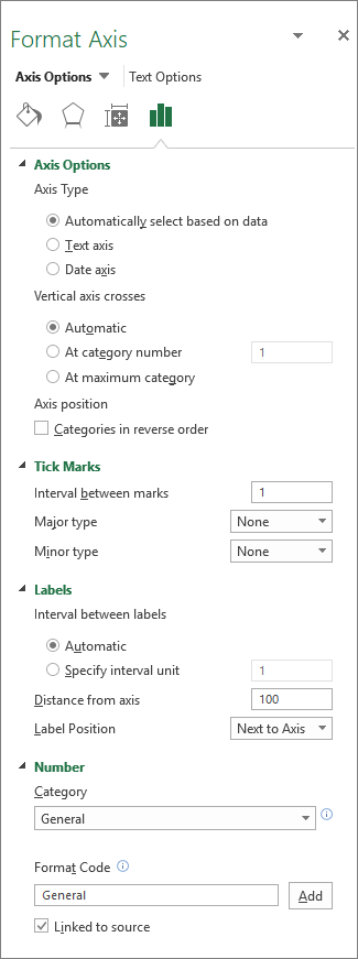
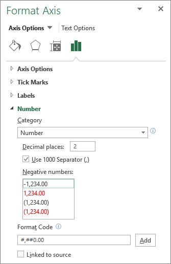
Under Axis Options, Click Number, and then in the Category box, select the number format that you want.
Tip If the number format you select uses decimal places, you can specify them in the Decimal places box.
To keep numbers linked to the worksheet cells, select the Linked to source check box.
Note Before you format numbers as a percentage, make sure that the numbers on the chart have been calculated as percentages in the source data, and that they are displayed in decimal format. Percentages are calculated on the worksheet by using the equation amount / total = percentage. For example, if you calculate 10 / 100 = 0.1, and then format 0.1 as a percentage, the number will be correctly displayed as 10%.
Change the display of chart axes in Office 2010
Click anywhere in the chart for which you want to display or hide axes.
This displays the Chart Tools, adding the Design, Layout, and Format tabs.
On the Layout tab, in the Axes group, click Axes.

Click the type of axis that you want to display or hide, and then click the options that you want.
On a chart, click the axis that has the tick marks and labels that you want to adjust, or do the following to select the axis from a list of chart elements:
Click anywhere in the chart.
This displays the Chart Tools, adding the Design, Layout, and Format tabs.
On the Format tab, in the Current Selection group, click the arrow in the Chart Elements box, and then click the axis that you want to select.
On the Format tab, in the Current Selection group, click Format Selection.
Under Axis Options, do one or more of the following:
To change the display of major tick marks, in the Major tick mark type box, click the tick mark position that you want.
To change the display of minor tick marks, in the Minor tick mark type drop-down list box, click the tick mark position that you want.
To change the position of the labels, in the Axis labels box, click the option that you want.
Tip To hide tick marks or tick-mark labels, in the Axis labels box, click None.
On a chart, click the horizontal (category) axis that you want to change, or do the following to select the axis from a list of chart elements:
Click anywhere in the chart.
This displays the Chart Tools, adding the Design, Layout, and Format tabs.
On the Format tab, in the Current Selection group, click the arrow in the Chart Elements box, and then click the axis that you want to select.
On the Format tab, in the Current Selection group, click Format Selection.
Under Axis Options, do one or both of the following:
To change the interval between axis labels, under Interval between labels, click Specify interval unit, and then in the text box, type the number that you want.
Tip Type 1 to display a label for every category, 2 to display a label for every other category, 3 to display a label for every third category, and so on.
To change the placement of axis labels, in the Label distance from axis box, type the number that you want.
Tip Type a smaller number to place the labels closer to the axis. Type a larger number if you want more distance between the label and the axis.
You can change the alignment of axis labels on both horizontal (category) and vertical (value) axes. When you have multiple-level category labels in your chart, you can change the alignment of all levels of labels. You can also change the amount of space between levels of labels on the horizontal (category) axis.
On a chart, click the axis that has the labels that you want to align differently, or do the following to select the axis from a list of chart elements:
Click anywhere in the chart.
This displays the Chart Tools, adding the Design, Layout, and Format tabs.
On the Format tab, in the Current Selection group, click the arrow in the Chart Elements box, and then click the axis that you want to select.
On the Format tab, in the Current Selection group, click Format Selection.
In the Format Axis dialog box, click Alignment.
Under Text layout, do one or more of the following:
In the Vertical alignment box, click the vertical alignment position that you want.
In the Text direction box, click the text orientation that you want.
In the Custom angle box, select the degree of rotation that you want.
Tip You can also change the horizontal alignment of axis labels, by right-clicking the axis, and then click Align Left , Center , or Align Right on the Mini toolbar.
You can change the text of category labels on the worksheet, or you can change them directly in the chart.
Change category label text on the worksheet
On the worksheet, click the cell that contains the name of the label that you want to change.
Type the new name, and then press ENTER.
Note Changes that you make on the worksheet are automatically updated in the chart.
Change the label text in the chart
In the chart, click the horizontal axis, or do the following to select the axis from a list of chart elements:
Click anywhere in the chart.
This displays the Chart Tools, adding the Design, Layout, and Format tabs.
On the Format tab, in the Current Selection group, click the arrow in the Chart Elements box, and then click the horizontal (category) axis.
On the Design tab, in the Data group, click Select Data.
In the Select Data Source dialog box, under Horizontal (Categories) Axis Labels, click Edit.
In the Axis label range box, do one of the following:
Specify the worksheet range that you want to use as category axis labels.
Tip You can also click the Collapse Dialog Box button  , and then select the range that you want to use on the worksheet. When you are finished, click the Expand Dialog Box button.
Type the labels that you want to use, separated by commas — for example, Division A, Division B, Division C.
Note If you type the label text in the Axis label range box, the category axis label text is no longer linked to a worksheet cell.
You can change the format of text in category axis labels or numbers on the value axis.
In a chart, right-click the axis that displays the labels that you want to format.
On the Mini toolbar, click the formatting options that you want.
Tip You can also select the axis that displays the labels, and then use the formatting buttons on the Home tab in the Font group.
In a chart, click the axis that displays the numbers that you want to format, or do the following to select the axis from a list of chart elements:
Click anywhere in the chart.
This displays the Chart Tools, adding the Design, Layout, and Format tabs.
On the Format tab, in the Current Selection group, click the arrow in the Chart Elements box, and then click the axis that you want to select.
On the Format tab, in the Current Selection group, click Format Selection.
Click Number, and then in the Category box, select the number format that you want.
Tip If the number format you select uses decimal places, you can specify them in the Decimal places box.
To keep numbers linked to the worksheet cells, select the Linked to source check box.
Note Before you format numbers as a percentage, make sure that the numbers on the chart have been calculated as percentages in the source data, and that they are displayed in decimal format. Percentages are calculated on the worksheet by using the equation amount / total = percentage. For example, if you calculate 10 / 100 = 0.1, and then format 0.1 as a percentage, the number will be correctly displayed as 10%.
Add tick marks on an axis
An axis can be formatted to display major and minor tick marks at intervals that you choose.
This step applies to Word for Mac only: On the View menu, click Print Layout.
Click the chart, and then click the Chart Design tab.
Click Add Chart Element > Axes > More Axis Options.
On the Format Axis pane, expand Tick Marks, and then click options for major and minor tick mark types.
After you add tick marks, you can change the intervals between the tick marks by changing the value in the Interval between marks box.
All about axes
Not all chart types display axes the same way. For example, xy (scatter) charts and bubble charts show numeric values on both the horizontal axis and the vertical axis. An example might be how inches of rainfall are plotted against barometric pressure. Both of these items have numeric values, and the data points will be plotted on the x and y axes relative to their numeric values. Value axes provide a variety of options, such as setting the scale to logarithmic.
Other chart types, such as column, line, and area charts, show numeric values on the vertical (value) axis only and show textual groupings (or categories) on the horizontal axis. An example might be how inches of rainfall are plotted against geographic regions. In this example, the geographic regions are textual categories of the data that are plotted on the horizontal (category) axis. The geographic regions will be uniformly spaced because they are text instead of values that can be measured. Consider this difference when you select a chart type, because the options are different for value and category axes. On a related note, the depth (series) axis is another form of category axis.
When you create a chart, tick marks and labels are displayed by default on axes. You can adjust the way that they are displayed by using major and minor tick marks and labels. To eliminate clutter in a chart, you can display fewer axis labels or tick marks on the horizontal (category) axis by specifying the intervals at which you want categories to be labeled, or by specifying the number of categories that you want to display between tick marks.
You can also change the alignment and orientation of the labels, and change or format the text and numbers that they display, for example, to display a number as a percentage.
Источник
A check mark is the universal character for confirmed tasks and is widely used in managing lists. Seeing how commonly it’s used in organizing ourselves, you would think that there should be a keystroke for this! In this article, we listed 5 methods you can use to to insert a check mark in Excel.
5 Methods to Add a Check Mark in Excel
Copy & Paste
Let’s start with the easiest method of adding a check mark in Excel. Copy & Paste the character below:
✓
Enjoy!
Symbols
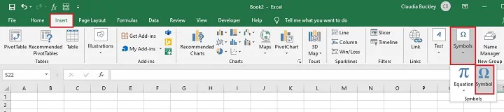
Excel (as well as Word) has a Symbol feature where all supported characters are listed. You can find the Symbol dialog from the INSERT > Symbols > Symbol path in the Ribbon.

In the Symbol dialog, choose Wingdings from the Font option, and scroll down to find the check mark character. Select the check mark and click the Insert button.

Alternatively, you can also type in 252 into the Character code box after selecting the Wingdings font. Knowing the symbol codes can expedite this process quite a bit.
Alt Code
You can enter any special character by typing in the corresponding code. All you need to do is to hold the Alt button, and type in the code. Since the check mark is a symbol that doesn’t exist in all font families, you need to set up the required font first.
Set a cell’s font type to Wingdings, and while holding the Alt key, press 0252 (the same code from the previous method) in the Symbol dialog.

CHAR Function
The CHAR function simply converts numeric codes into the equivalent ANSI character. For example, the =CHAR(252) formula returns the equivalent character (a check mark) for selected font type. The Wingdings font type should be selected for the check mark to be recognized.

Conditional Formatting
The Conditional Formatting feature can add icons into cells based on cell values and you can use this feature to add a check mark in Excel. For example, you can set rules like «if the cell is equal to 1, then put a check mark».
To apply Conditional Formatting follow the steps below:
- Select the range you want place check marks.
- Go to HOME > Conditional Formatting > Icon Sets and click the set with check mark.
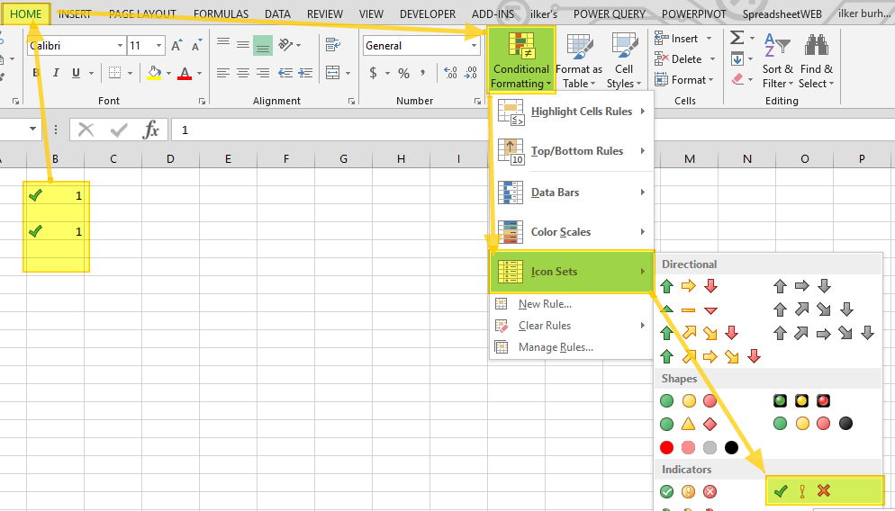
By default, check marks are associated with ones (1) and crosses with zeros (0). The default rule also calculates the percentiles of the selected range and places check marks for the highest 1/3 of values. To update this rule, click the Manage Rules button under the Conditional Formatting menu while the data range is selected. This will bring up the Conditional Formatting Rules Manager. Double-click on the appropriate rule to edit it. Here you can,
- Remove or change other symbols.
- Place check marks for a certain numbers.
- Hide the cell values, and only show the icons.
Check marks have become a part of our task-oriented lives. If you use Excel to generate and execute lists (and you probably do), inserting an Excel check mark symbol will come in mighty handy. In this tutorial, we’ll show you how to insert a check mark in Excel.
What is a check mark?
A check mark or tick (✓) is a symbol that is universally associated with a positive response (for example, yes, completed, correct, etc.). The tick symbol in Excel is treated as text. This means that the color and size can be changed like any other text would be, and the location can be changed using the standard Copy and Paste commands.
Check marks are not the same as check boxes. A check box in Excel is an object which is placed on a worksheet. A check box that appears to be in a cell will not be deleted if that cell is deleted, because the check box is not actually a part of the cell. The location of a check box can be changed by dragging it as you would any other object.
Download your free check mark practice file!
Use this free Excel check mark file to practice along with the tutorial.
How to insert a check mark
There are multiple ways to insert a check mark in Excel. Five commonly-used methods are shown below.
Method 1: Shift P, Wingdings 2 font
A check mark is just another text character. If you can remember that SHIFT + P is that character, you can simply type an uppercase P in your desired cell, and change the font to Wingdings 2 as you would perform any regular font change. The Wingdings check mark will then be displayed in the worksheet.
 You may also care to know that SHIFT + O in the Wingdings 2 font inserts the X symbol (×).
Method 2: Insert — symbol menu
The Excel ribbon has an Insert tab, and from there a Symbol dropdown. Choose the Symbol command and you will find all the supported symbols in Excel.
 In the Symbol dialog box, choose the Wingdings font option, and scroll down to find the check mark character.
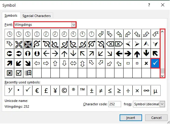 Select the check mark and click the Insert button to place the check mark in the worksheet, then click Close to close the dialog window.
You can see in the above image that Excel stores recently used symbols toward the bottom of the Symbol dialog box to save time if you need to insert them again.
Method 3: ALT 0252
If you saw the character code 252 at the bottom of the dialog box in the previous method, this might be a good reminder of an Excel check mark shortcut.
You’ll need to change the font to Wingdings, then hold the ALT button while typing in 0252. Note that the numbers should be entered from the numeric pad on the keyboard, and not from the QWERTY numbers above the letters.
 If you forgot to change the font to Wingdings before doing the ALT 0252 shortcut, you may see a character that looks like this: ü. No worries. Just change that cell to the Wingdings font and your check mark will be displayed.
Note: There is no such option on Mac devices.
Method 4: UNICHAR function
A check mark can be inserted using a function? Yes, it can. UNICHAR is a text function that returns the character represented by the Unicode argument in parentheses. Remember that each character is assigned a special code within the computer’s memory. Once you know the code for the character you want to insert, you can use UNICHAR to insert it.
=UNICHAR(10003) inserts a check mark, and UNICHAR(10004) inserts a heavy check mark.
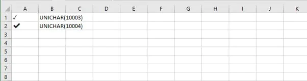 This method offers the advantage of not having to change to a special font. If you choose to use the UNICHAR function, bear in mind that the check mark has to be the only value in that cell.
UNICHAR(10007) and UNICHAR(10008) will insert the X and heavy X, respectively.
Method 5: Conditional formatting
Conditional formatting tells cells how to behave if certain conditions are met. The Conditional Formatting feature can add icons into cells based on cell values, and you can use this feature to add a check mark in Excel.
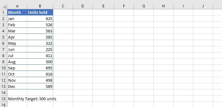
For example, download the practice file and work along while we use conditional formatting to insert a check mark next to each month where the target of 500 unit sales per month was met, and an X next to the months where the target was not met.
Download your free check mark practice file!
Use this free Excel check mark file to practice along with the tutorial.
To apply conditional formatting, follow the steps below:
- Select the range where you want to place check marks (B2 to B13).
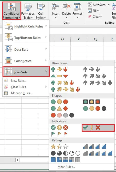
- Go to the Home tab > click Conditional Formatting > then choose Icon Sets and select the set which includes the check mark indicator. This will be a 3-symbol icon set (a check mark, an X, and an exclamation mark).
 By default, Excel places a check mark for values within the 67th percentile and higher, and an X for values below the 33rd percentile. For values between the 33rd and 66th percentiles, an exclamation symbol is the default.
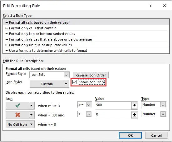
- Change this default rule by going to the Manage Rules button under the Conditional Formatting menu while the data range is selected. This will bring up the Conditional Formatting Rules Manager window. Click the Edit Rules command to change the conditions under which these symbols are applied.
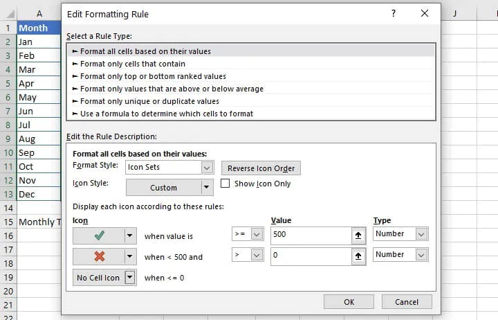
- In the lower third of the Edit Formatting Rule window, change Percent to Number under the Type dropdown, and change the value 67 to 500. This will cause cells that are greater than or equal to 500 to have a check mark inserted.
- Just below that, change the exclamation symbol to an X from the Icon dropdown, change the >= symbol to >, the Type to Number, and the Value to 0.
- For the third symbol, click the dropdown and select No cell icon.
- Click OK to confirm your changes and OK to apply them and return to the worksheet.
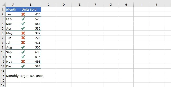 You will now be able to tell at a glance whether the monthly target was met or not.
There is also the option of displaying the symbols only, without the associated number. Do this by returning to the Conditional Formatting Rules Manager, choosing Edit Rule, and then selecting the Show Icon Only checkbox.
 When applied, the cells will now display the icons only.
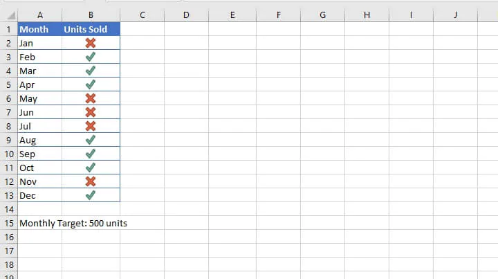 Of course, since the check mark behaves just like a text character, you can make it bold, color it, increase the font size, change the alignment, and apply any other text formatting you like.
Learn more
Easy breezy. If you’ll be using check marks in Excel often, decide on your one or two favorite methods and practice them.
Like what you learned? Try the GoSkills range of Excel courses to see what else you can learn in Excel. You can try our Microsoft Excel — Basic and Advanced course. Or start with our free Excel in an Hour course to learn some basics in Excel.
Learn Excel for free
Start learning formulas, functions, and time-saving hacks today with this free course!
Start free course