
Excel for Microsoft 365 Excel 2021 Excel 2019 Excel 2016 Excel 2013 Excel 2010 Excel 2007 More…Less
In Excel, formatting worksheet (or sheet) data is easier than ever. You can use several fast and simple ways to create professional-looking worksheets that display your data effectively. For example, you can use document themes for a uniform look throughout all of your Excel spreadsheets, styles to apply predefined formats, and other manual formatting features to highlight important data.
A document theme is a predefined set of colors, fonts, and effects (such as line styles and fill effects) that will be available when you format your worksheet data or other items, such as tables, PivotTables, or charts. For a uniform and professional look, a document theme can be applied to all of your Excel workbooks and other Office release documents.
Your company may provide a corporate document theme that you can use, or you can choose from a variety of predefined document themes that are available in Excel. If needed, you can also create your own document theme by changing any or all of the theme colors, fonts, or effects that a document theme is based on.
Before you format the data on your worksheet, you may want to apply the document theme that you want to use, so that the formatting that you apply to your worksheet data can use the colors, fonts, and effects that are determined by that document theme.
For information on how to work with document themes, see Apply or customize a document theme.
A style is a predefined, often theme-based format that you can apply to change the look of data, tables, charts, PivotTables, shapes, or diagrams. If predefined styles don’t meet your needs, you can customize a style. For charts, you can customize a chart style and save it as a chart template that you can use again.
Depending on the data that you want to format, you can use the following styles in Excel:
-
Cell styles To apply several formats in one step, and to ensure that cells have consistent formatting, you can use a cell style. A cell style is a defined set of formatting characteristics, such as fonts and font sizes, number formats, cell borders, and cell shading. To prevent anyone from making changes to specific cells, you can also use a cell style that locks cells.
Excel has several predefined cell styles that you can apply. If needed, you can modify a predefined cell style to create a custom cell style.
Some cell styles are based on the document theme that is applied to the entire workbook. When you switch to another document theme, these cell styles are updated to match the new document theme.
For information on how to work with cell styles, see Apply, create, or remove a cell style.
-
Table styles To quickly add designer-quality, professional formatting to an Excel table, you can apply a predefined or custom table style. When you choose one of the predefined alternate-row styles, Excel maintains the alternating row pattern when you filter, hide, or rearrange rows.
For information on how to work with table styles, see Format an Excel table.
-
PivotTable styles To format a PivotTable, you can quickly apply a predefined or custom PivotTable style. Just like with Excel tables, you can choose a predefined alternate-row style that retains the alternate row pattern when you filter, hide, or rearrange rows.
For information on how to work with PivotTable styles, see Design the layout and format of a PivotTable report.
-
Chart styles You apply a predefined style to your chart. Excel provides a variety of useful predefined chart styles that you can choose from, and you can customize a style further if needed by manually changing the style of individual chart elements. You cannot save a custom chart style, but you can save the entire chart as a chart template that you can use to create a similar chart.
For information on how to work with chart styles, see Change the layout or style of a chart.
To make specific data (such as text or numbers) stand out, you can format the data manually. Manual formatting is not based on the document theme of your workbook unless you choose a theme font or use theme colors — manual formatting stays the same when you change the document theme. You can manually format all of the data in a cell or range at the same time, but you can also use this method to format individual characters.
For information on how to format data manually, see Format text in cells.
To distinguish between different types of information on a worksheet and to make a worksheet easier to scan, you can add borders around cells or ranges. For enhanced visibility and to draw attention to specific data, you can also shade the cells with a solid background color or a specific color pattern.
If you want to add a colorful background to all of your worksheet data, you can also use a picture as a sheet background. However, a sheet background cannot be printed — a background only enhances the onscreen display of your worksheet.
For information on how to use borders and colors, see:
Apply or remove cell borders on a worksheet
Apply or remove cell shading
Add or remove a sheet background
For the optimal display of the data on your worksheet, you may want to reposition the text within a cell. You can change the alignment of the cell contents, use indentation for better spacing, or display the data at a different angle by rotating it.
Rotating data is especially useful when column headings are wider than the data in the column. Instead of creating unnecessarily wide columns or abbreviated labels, you can rotate the column heading text.
For information on how to change the alignment or orientation of data, see Reposition the data in a cell.
If you have already formatted some cells on a worksheet the way that you want, there are several ways to copy just those formats to other cells or ranges.
Clipboard commands
-
Home > Paste > Paste Special > Paste Formatting.
-
Home > Format Painter
 .
.
 .
.Right click command

-
Point your mouse at the edge of selected cells until the pointer changes to a crosshair.
-
Right click and hold, drag the selection to a range, and then release.
-
Select Copy Here as Formats Only.
Tip If you’re using a single-button mouse or trackpad on a Mac, use Control+Click instead of right click.
Range Extension
Data range formats are automatically extended to additional rows when you enter rows at the end of a data range that you have already formatted, and the formats appear in at least three of five preceding rows. The option to extend data range formats and formulas is on by default, but you can turn it on or off by:
-
Newer versions Selecting File > Options > Advanced > Extend date range and formulas (under Editing options).
-
Excel 2007 Selecting Microsoft Office Button
> Excel Options > Advanced > Extend date range and formulas (under Editing options)).
 > Excel Options > Advanced > Extend date range and formulas (under Editing options)).
Need more help?

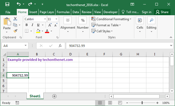
This Excel tutorial explains how to format the display of a cell’s text in Excel 2016 such as numbers, dates, etc (with screenshots and step-by-step instructions).
Question: How do I format how the text displays in a cell in Microsoft Excel 2016?
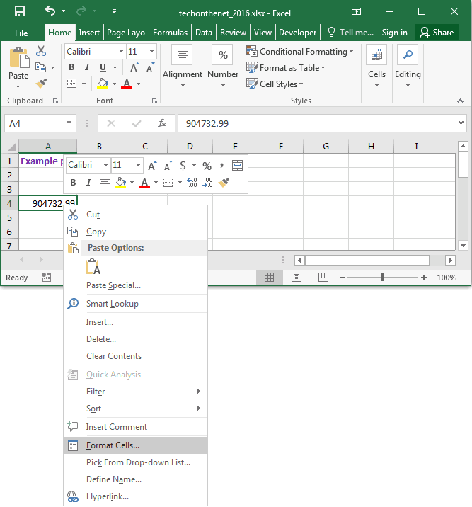
Answer: Select the cells that you wish to format.
Right-click and then select «Format Cells» from the popup menu.
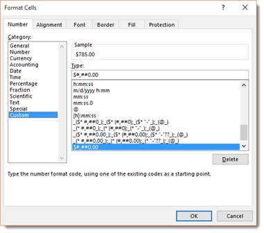
When the Format Cells window appears, select the Number tab. In the Category listbox, select your format. A sample of your text will appear on the right portion of the window based on the format that you’ve selected. Click the OK button when you are done.
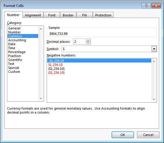
In this example, we’ve chosen to format the content of the cells as a currency number with 2 decimal places.
Font is defined as the style of your type. Times New Roman, Courier, and Arial are probably three of the most popular fonts, but there are literally hundreds. When you create a worksheet, you can decide what type of font you want to use. You can also decide the size of the font.
In the snapshot below, we’ve used Calibri, size 11 font.
However, we can change that to another font and another size.
To change the font type and size, go to Font group under the Home tab.
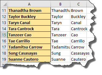
Next, select the data in the worksheet for which you want to change the font. We’ve selected column A in the snapshot below.
Go to the Font group, and you’ll see the type of font that you’re currently using. It appears in a box with a downward arrow beside it on the left hand side of the toolbar. In our example, and on our toolbar, it’s Calibri.
Click on the downward arrow to the right font type and select a new font.
We’re going to select Arial.
Once you select the font, the selected data will be changed to the new font.
To change the size, select the cells, then click the downward arrow beside the current size.
You may want to select boldface, italicize, or underline data inside cells. The boldface command in MS Excel is represented by an uppercase, boldfaced B. Italics are represented by an uppercase, italicized ‘I’, and underline by an uppercase U with a line under it. These buttons are located directly below the font type window in the Font group.
To add italics, boldfaced, or underlining to data in cells, select the desired cells, then click the appropriate button (B for boldfaced, I for italic, or U for underline).
By clicking the downward arrow to the right of the underline button, you can choose an underline style.
You can choose the standard underline, which is a single line. You can also choose the double underline, which is two lines.
You can also add borders to cells or a range of cells by selecting the cell(s) you want to add border to, then by clicking Border button in the Font group under the Home tab.
Simply select where you want to border to appear and what kind of border you want. Keep in mind that the border you choose will be applied to a single selected cell or to a range of selected cells.
You can also change the line color of the border and the border style (such as dashed or solid lines) by going to the Draw Borders section of the dropdown menu.
Let’s see how it works.
We want to apply borders to the cells in column A.
As you can see below, we’ve selected the cells.
Next, we go to the Ribbon and click the Borders button.
We choose Thick Outside Borders.
Since we selected a range of cells, the border is applied to the entire range, not the individual cells.
Let’s do something a little different now. Instead of applying a border, we’re going to go to the Draw Borders section of the dropdown menu. We’re going to draw borders.
Select Draw Border from the dropdown menu.
When you draw a border, your mouse cursor turns into a pencil. You can click the border of a cell to add a border. You can also drag your mouse over cells to add a border. We are going to drag our mouse over column C.
You can also choose to add a line color or a line style for the border you draw. We’re going to choose Line Color from the dropdown menu, and choose the color red. Once again, you can click the border of a cell to add a border. You can also drag your mouse over cells to add a border.
Changing the font color is as easy to do as changing the font. By default, your text in Excel 2016 appears in a black font. If you want to change the font color, look for the uppercase A with a colored bar under it in the Font group under the Home tab.
Select the cells for which you want to change the font color, then click on the button to choose the color you want to apply to the selected text.
You can also add color to a cell or range of cells. This doesn’t change the font color, but instead provides a colored background.
To the left of the font color button, you’ll see what looks like a paint bucket with a yellow bar underneath it. Simply select the cells you want to give a color, click the button, and select the color of highlight that you want to apply.
In the example below, we chose a yellow.
Please note that the cell borders that show up in Excel by default are no longer displayed when we add color. If you want borders, you have to add them.
We selected All Borders from the Borders dropdown menu, then dragged over the cells in column A to apply the borders.
The Format Cells Dialogue Box
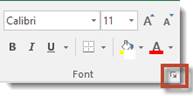
Click the arrow in the right side bottom corner of the Font group to access the Format Cells dialogue box.
The dialogue box looks like this:
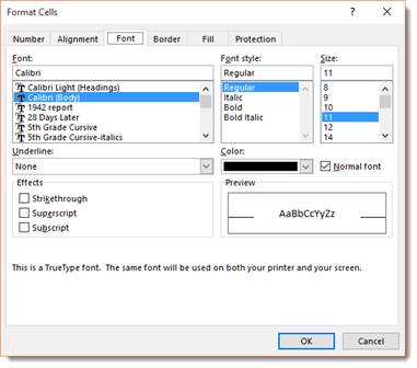
From this dialogue box, you can format your data just as you did from the Ribbon. The Preview section of the dialogue box lets you preview your changes before you apply them.
Click OK when you’re finished making changes to apply them to your spreadsheet.
Formatting with the Mini-Bar
The mini-bar appears whenever you right click within a cell.
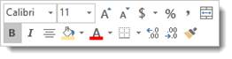
In the snapshot above, you can see that it contains the tools to change the font, font size, etc. You can use this to format your cells to save the time you’d spend going to the Ribbon.
Merge Cells
Merging cells simply means that you merge a group of cells into one cell. It is not the same as combining cells because when you combine cells, the data in those cells is also combined.
When you merge cells, the information in the upper left cell is centered in the merged cell. If the content you want in the merged cells is not in the upper left cell, then you must copy and paste the data into the upper left cell.
Note: It’s important to remember that the cells you merge must be adjacent. In addition, the cells that you merge cannot be active or the Merge and Center feature will not work.
To merge cells, first select the cells to be merged.
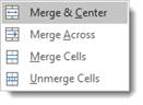
Go to the Alignment group under the Home tab, then click Merge and Center.
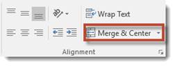
Select an option from the dropdown menu.
Apply Number Formats and Create Custom Number Formats
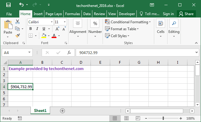
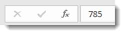
You can change the appearance of numbers in MS Excel 2016 without changing the value behind those numbers. The actual value is always displayed in the Formula Bar.
For example, we can have a numbers formatted as currency in the worksheet:
Yet, if we click on a cell in the Formula Bar, the number is displayed as a general number.
You can apply a number format to a cell by selecting the cell(s) that you want to format, right clicking, and selecting Format Cells and select the Number tab.
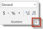
You can also to the Home tab, go to the Number group, then click on the arrow in the bottom right corner.
You will then see the Format Cells dialogue box. Click on the Number tab.
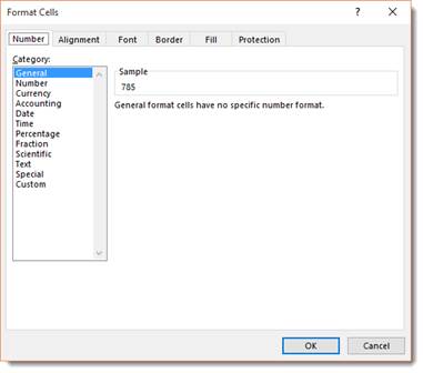
In the dialogue box above, you can choose the type of number formatting that you want from the Category column. An explanation of how the formatting is used appears at the bottom of the dialogue box when you click on a specific type of number formatting.
We chose Currency from the Category column.
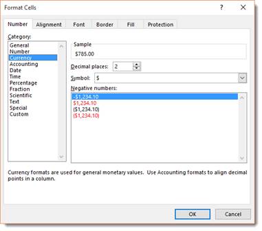
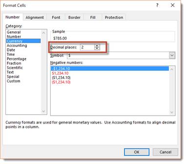
We wanted two numbers to appear after the decimal point.
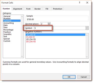
We wanted to use the American dollar symbol.
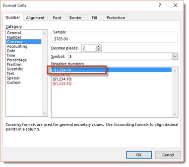
We wanted negative numbers to appear with the minus (-) sign before them. We could have also chosen to have them appear in red, black with parentheses, or red with parentheses.
Click Ok when you’re finished.
Creating Custom Number Formatting
If the number formats the Excel provides won’t work for your data, you can create a custom number format. To do this, go to the Format Cells dialogue box again, and click Custom n the category column.
In the Type list, select the format that you want to customize. As you can see in the snapshot above, we chose the currency format.
Now go to the Type field and customize the format by entering the format you want to use.
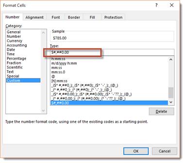
Click OK when you’re finished.
Align Cell Contents
You can align the data in a cell to the left, right, or center.
To align data to the left means to align it to the left side of the cell. Simply select the cell(s) that contain the data that you want to align to the left.
Go to the Alignment group under the Home tab.
Click:
 To align to the left.
 To align to the right.
 To align to the center.
 To align data to the top of a cell.
 to align data to the middle of the cell.
 To align data to the bottom of the cell.
About Indents
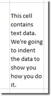
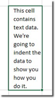
You can also indent data in cells. When you increase indent, you increase the margin between data in the cell and the left cell border.
The cell pictured below has text data in it.
Select the cells that contain data that you want to indent. Then, go to the Alignment group under the Home tab.
The two buttons highlighted below allow you to decrease indent (first button), or increase indent.
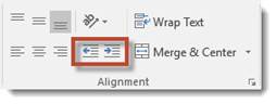
We’re going to increase the indent (second button).
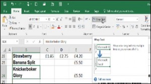
About Text Wraps
Text wrap will wrap the entries from selected cells that have data that spills over their right borders.
Here’s an example:

Select the cell(s) you want to apply text wrap to, then click the Wrap Text button in the Alignment group under the Home tab.

The text is then wrapped within the cell.
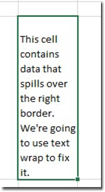
As you can see, the text is now wrapped to fit between the left and right borders of the cell.
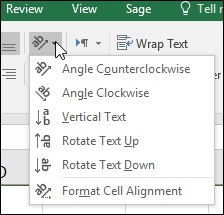
Changing the Orientation of Cell Entries
Instead of wrapping text in cells, you can also change the orientation of the text by rotating the text up or down. This can work well with labels in worksheets.
In the example below, we’re going to change the orientation of the data that contains the days of the week.
To start with, we’ve selected the cells that contain this data:

Next, we go to the Alignment group under the Home tab and click the Orientation button. It looks like this:

From the Orientation dropdown menu, we now we get to choose the new orientation:
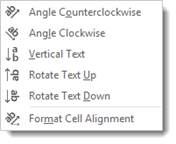
We’re going to choose Rotate Text Up.
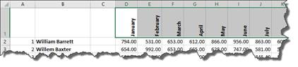
You can see that our column labels are now vertical with the text going upward (from bottom to top).
The Format as Table Gallery
The Format as Table Gallery is a way to format your cells without having to select the cells first. Think of it as a shortcut to formatting cells. Your cell cursor just has to be within the table of data right before you click the Format as Table button that’s located in the Styles group under the Home tab (pictured below).
We’re going to put our mouse cursor in a cell by clicking on the cell.
Now we’re going to go to the Format as Table button and look at the gallery.
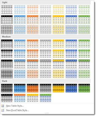
Choose a formatting style that you want.
When you click on a style that you want, you’ll see the Format as Table dialogue box.
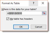
This contains the cells referenced for the formatting. In the dialogue box pictured above, Excel has the referenced cells listed as D1 through O10. If this is incorrect, you can change it.
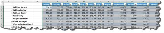
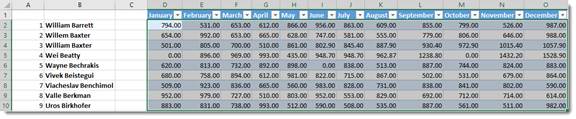
Put a checkmark beside «My table has headers» if your data has headers. Ours does. The headers are the column labels. In our example, the headers are the months of the year.
Click OK when you’re finished.
The Table Tools Design tab then opens in the Ribbon.

Located under the Table Tools Design tab is a Table Styles Options group that allow you customize your table even further.
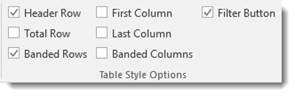
Header Row adds formatting and filter buttons to each of the headings in the first row. Ours already has filter buttons (the down arrow)
-
Total Row goes at the bottom of the table for totals.
-
Banded Rows means shading will be applied to every other row.
-
First Column puts row headings in the first column in boldface.
-
Last Column puts row headings in the last column of the table in boldface.
-
Banded Columns applies shading to every other column.
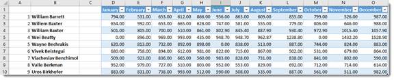
In the Table Styles group, you can also change the style of table that you applied when you chose a format for your table from the gallery.
Our table now looks like this:
Conditional Formatting
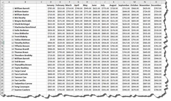
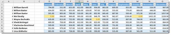
Conditional formatting is a neat little feature of Excel 2016 because it helps you do your job better. Let’s say that you’re entering in sales figures for each employee into a spreadsheet. Your boss has told you to let him know if anyone sells less than $300.00 worth of products in a given month. Did you know that you Excel can notify you each time this happens? You can program Excel 2016 to give you a «red flag» every time a certain situation exists.
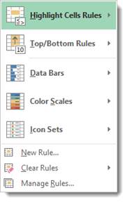
To apply conditional formatting, go to the Styles group under the Home tab. Click the Conditional Formatting button. You will see a dropdown menu.
Let’s learn what each of the options does for you:
-
Highlight Cells Rules allows you to define rules that highlight the cells in the cell selection when certain values such as text or dates that have greater or less than a value that you specify or fall within a range of values.
-
Top/Bottom Rules gives you options for defining rules that highlight the top and bottom values, percentages, and above and below average values in a cell selection.
-
Data Bars opens a palette with different colors of data bars. You can apply these to a cell selection to indicate their values relative to each other.
-
Color Scales opens a palette with different color scales that you can apply to a cell selection to indicate their values relative to each other.
-
Icon Sets will open a palette with icons. You can apply these icons to a cell selection to indicate values relative to each other by clicking the color scale thumbnail.
-
New Rule allows you to create new rules.
-
Clear Rules allows you to remove conditional formatting rules for the cell selection.
-
Manage Rules opens a dialogue box where you can edit and delete rules.
Let’s apply conditional formatting to our spreadsheet.
We’re going to use Highlight Cell Rules.
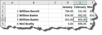
First, we select the cells. This is our cell selection.
Now, we go to the Conditional Formatting button on the Ribbon and choose Highlight Cell Rules.
We want to cells to be highlighted when a value is less than 300. We chose Less Than from the side menu that appears when you click Highlight Cell Rules.
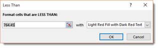
We want to format cells that are less than 300, so we’re going to enter that into the box.
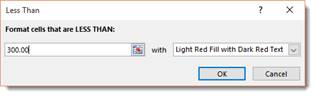
Next, we choose what colors we want to use to highlight the cells that have values less than $300.
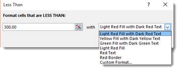
We are going to choose Yellow Fill with Dark Red Text.
Click OK when you’re finished.
As you can see in our snapshot below, the cells less than 300.00 are now highlighted.
Creating and Applying Styles
If you frequently use the same formatting options for the cells in your worksheets, you may want to create a formatting style to save you time. A formatting style is a collection of formatting choices. It may include— but not be limited to— font, font size, and color.
To create a new style, first format a cell with the selection of styles that you want.
Select the cell.
We’ve selected the cell below as our example:
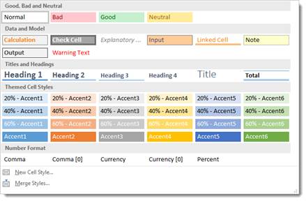
Next, go to the Home tab to the Styles group, and click the downward arrow to the right of the Styles gallery.
Select New Cell Style from the dropdown menu.
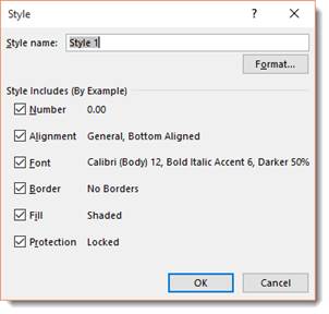
Create a name for the style in the Style Name field, then choose the formatting options that you want to include in the style.
Click OK when you’re finished.
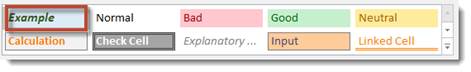
As you can see, our new style now appears as the first style on the left in the Style Gallery.
NOTE: You can also apply pre-created styles from the Style Gallery and apply them to cells or ranges of cells. To apply a style, select a cell or range of cells, then choose the style from the gallery that you want to apply.
Formatting Using Quick Analysis
Quick Analysis is a feature that was new to Excel 2013. It can make doing things such as creating charts, adding sums, or even formatting cells easier than ever before. In fact, you can do it in as little as two clicks of the mouse.
To format cells using Quick Analysis, first select the cells that you want to format.
When you select your cells, you’ll see the Quick Analysis button appear at the bottom right of the selection. We highlighted it in red below.
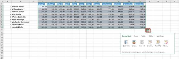
Click on it and the Quick Analysis tool opens. We have now highlighted it in red.
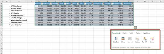
Let’s zoom in and get a better look at it:
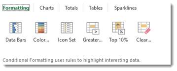
By default, Formatting options are shown to you when you click on the tool. From here, you can apply conditional formatting the same way as we learned to do earlier in this lesson. You can also work with charts, totals, tables, and sparklines.
The Format Painter
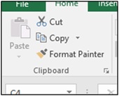
The Format Painter tool is located under the Home tab in the Clipboard group.
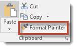
The Format Painter looks like a broom, but it acts more like a paintbrush.
Using it, you can «borrow» the formatting from cells or selections of cells and apply the same formatting somewhere else. It’s operates a lot like the «copy» function in Excel, except instead of copying text, you’re copying formatting.
To use the Format Painter, select the cell or cells for which you want to copy formatting.
Now, click the Format Painter button. You’ll notice that the cursor changes to a paintbrush.
Next, select the cell(s) you want to change to paint with the borrowed format.
Creativity and uniformity are few of the least aspects most people consider in using Excel. More often, we tend to disregard the styles we use, for instance fonts, no matter how different they are from each other. We ignore the format, most especially when we are working with lots of information in a worksheet. However, formatting your worksheets is not a difficult task at all. Doing so will make your file look more organized and professional. Uniformity will even encourage you to work on your file with enthusiasm and excitement.
The Home Ribbon to customize and format cells and worksheets
Excel 2016 consists of several ribbons that make you do complicated tasks in just few clicks. One of them is the Home Ribbon. This portion contains mostly of formatting and editing tools.
The Main Groups in Excel 2016 Home Ribbon
1. Font Group
This group contains the main features for changing the appearance of your content, as shown below.
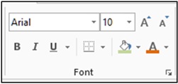
Using the font group, you will be able to change the font style and size of the contents of your cell. Just follow the steps below.
- Go to Home Ribbon and look for the Font Group.
- Select the cell/s you want to format.
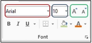
- Click on the drop down arrow next to the font style (red) or font size (blue) box.
- Select the font style or font size you require.
Note: Changing the font size is also possible just by clicking the “grow and shrink font” button, enclosed in green.
You can also make your contents be boldfaced, italicized or underlined in just a click.
- Select the cell/s you want to format.
- Click on the icon you require.
![]()
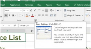
For more detailed changes, you can explore the font settings by following the steps below.
- Select the cell/s you want to format.
- Click on the Dialog box launcher arrow.
- Make the changes you require.
- Click OK.
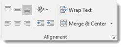
2. Alignment Group
This group indicates where your text/numbers will line up in a cell.
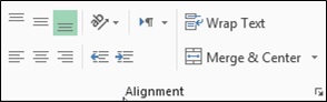
Setting the Alignment
- Click on the cell/s you want to format.
- Click on the icon you require.

Text/ Number Orientation
You can also change the direction of text in a cell/s by simply selecting the cell/s to change and then choose the orientation you need.
3. Number Group
Number group allows formatting of your figures. It has shortcuts for a particular number format, like adding currency – which could be GBP, Dollars or the Euro symbol, formatting a number as a percentage, adding a thousand separator or increasing/ decreasing decimals.
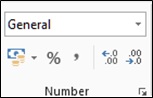
To apply number format
- Select the cell/s you want to format.
- Click the drop down arrow.
- Choose the format you need.
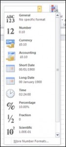
To remove number format
- Select the cell/s you want to clear the format.
- Click the drop down arrow.
- Choose the first option – General (No Specific Format).
Other Important Features…
4. Wrap Text
This feature helps you add more text in the cell by increasing its height but keeping its width. It is useful if you have text that is too wide for the cell.
- Select the cell you want to wrap.
- Go to the Alignment Group on the Home Tab.
- Click on Wrap Text button.
5. Format Painter
This feature allows you to copy the formatting from one part of your workbook to another.
Using Format Painter Once
- Select the cell that contains the formatting you want to copy.
- In the Clipboard group of the Home ribbon, click on the Format Painter button.
- Click on the cell (or click and drag on the cells) you want to apply the formatting.
Using Format Painter to copy to more than one cell
- Select the cell that contains the formatting you want to copy.
- In the Clipboard group of the Home ribbon, double click the Format Painter button.
- Click and drag over the text you want to use the format with.
- Click on the Format Painter button once again to switch it off.
Formatting your calls and worksheets is not hard at all. The Home Ribbon allows you to do it in just a few clicks. You will only have to select the cell/s you want to format, then click on the command button you need – it’s just that simple!
We have even more useful articles:
Excel 2016: 3 Simple Steps to Hide and Unhide Portions
“Essential Facts About Worksheets and Workbooks and How to Utilize Them”
“Customize The ‘Quick Access Toolbar”
“How to Use Excel’s Basic Functions”
Условное форматирование представляет собой гибкий и практичный способ применения форматирования ячеек в индивидуальном или групповом порядке на основе их значений. В качестве примера, вы можете настроить условное форматирование так, чтобы все ячейки с числовыми значениями меньше 0 были окрашены в красное. Во время ввода или изменения значения ячейки Excel осуществляет его проверку и сравнение с условиями, которые заданы в правилах. Если значение будет меньше нуля, фон поменяется на красный, в противном случае цвет не изменится.
По сути, условное форматирование позволяет легко идентифицировать ячейки с некорректными значениями либо записями соответствующего типа.
Как применить условное форматирование в Excel 2016, 2013, 2010, 2007?
Все нужные нам составляющие находятся в разделе меню «Условное форматирование» в категории «Стили» на вкладке «Главная».

Вот какие опции тут доступны:
- правила выделения ячеек. Тут можно задать условия форматирования на основе значений ячеек и их величин. Наиболее часто используемая опция
- правила отбора первых и последних значений. Предоставляет возможности, связанные с заданием формата ячеек на основе их вхождения в топ первых или последних величин
- гистограммы. Пожалуй, наиболее мощное из средств визуализации форматирования, наряду с цветовыми шкалами и наборами значков. Предоставляет палитру гистограмм всевозможных оттенков, которые вы можете задавать для величин ячеек
- цветовые шкалы. Обеспечивает возможность задания двух- и трехцветовых шкал, доступных для цвета фона ячейки на базе ее величины в сравнении с другими ячейками в диапазоне
- наборы значков. Позволяет отобразить в ячейке значок. Рисунок отображаемого значка зависит от величины ячейки в сравнении с другими ячейками. На выбор пользователя предоставляется до 20 наборов значков, которые вы можете комбинировать между собой.
Применим в качестве примера форматирование к диапазону ячеек, чтобы их цвет менялся в зависимости от значения. Как это сделать? Для этого нам придется создать несколько правил.
Вначале выделим диапазон ячеек, к которому мы хотим применить форматирование. Это может быть как целый лист, так и выбранная область.

Итак, первое правило: если значение ячейки меньше нуля, ее фон должен окрашиваться в красный. Реализуем это на практике. Выбираем на ленте опцию «Условное форматирование» -> «Правила выделения ячеек» -> «Меньше».

Появляется мини-форма с указанием условия, на основе которого будет сформировано правило. Поскольку нам нужно условие «меньше 0», то вставляем цифру 0 в левой части формы. Справа же выбираем расцветку фона, которую мы хотели бы видеть на соответствующих ячейках. Также тут в дополнение можно указать цвет текста.

Создадим еще одно правило: если значение ячейки больше 0, окрашиваем ее в желтый цвет. На этот раз выберем правило «Больше».

Наконец, последнее третье правило: если значение равно 0, преобразуем цвет в зеленый.

Теперь вводим числа в указанный диапазон и созерцаем результат.

Как применить условное форматирование в Excel 2003?
В ранних релизах Экселя возможности условного форматирования гораздо ниже. Так, тут полностью отсутствуют такие средств визуализации, как гистограммы, цветовые шкалы и наборы значков, а все, на что способен встроенный модуль – это принять простейшие условия, наподобие тех, о которых шла речь выше.
Опция условного форматирования в Excel 2003 скрыта в разделе главного меню «Формат».

Это был лишь самый простой пример условного форматирования, Excel способен на гораздо большее. Тем не менее, общее представление об этом функционале из данной статьи вам получить все же удастся.
Показать видеоинструкцию
Видеоинструкция
Ответы на другие вопросы: