
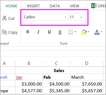
Change font style, size, color, or apply effects
Click Home and:
-
For a different font style, click the arrow next to the default font Calibri and pick the style you want.
-
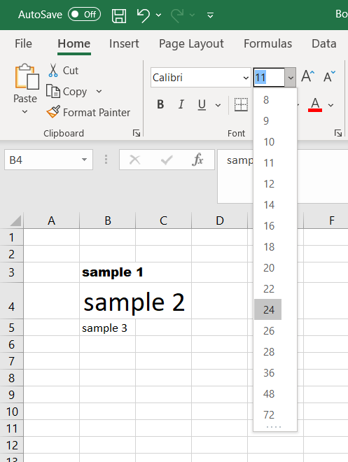
To increase or decrease the font size, click the arrow next to the default size 11 and pick another text size.

-
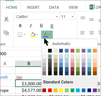
To change the font color, click Font Color and pick a color.
-
To add a background color, click Fill Color next to Font Color.
-
To apply strikethrough, superscript, or subscript formatting, click the Dialog Box Launcher, and select an option under Effects.
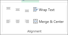
Change the text alignment
You can position the text within a cell so that it is centered, aligned left or right. If it’s a long line of text, you can apply Wrap Text so that all the text is visible.
Select the text that you want to align, and on the Home tab, pick the alignment option you want.
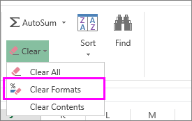
Clear formatting
If you change your mind after applying any formatting, to undo it, select the text, and on the Home tab, click Clear > Clear Formats.
Change font style, size, color, or apply effects
Click Home and:
-
For a different font style, click the arrow next to the default font Calibri and pick the style you want.
-
To increase or decrease the font size, click the arrow next to the default size 11 and pick another text size.
-
To change the font color, click Font Color and pick a color.
-
To add a background color, click Fill Color next to Font Color.
-
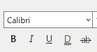
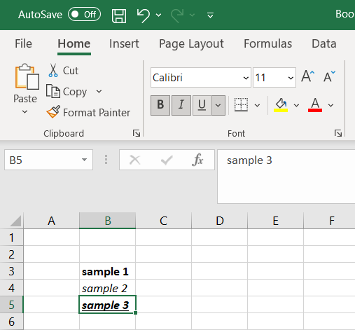
For boldface, italics, underline, double underline, and strikethrough, select the appropriate option under Font.

Change the text alignment
You can position the text within a cell so that it is centered, aligned left or right. If it’s a long line of text, you can apply Wrap Text so that all the text is visible.
Select the text that you want to align, and on the Home tab, pick the alignment option you want.
Clear formatting
If you change your mind after applying any formatting, to undo it, select the text, and on the Home tab, click Clear > Clear Formats.
Format Fonts
You can format fonts in four different ways: color, font name, size and other characteristics.
Font Color
The default color for fonts is black.
Colors are applied to fonts by using the «Font color» function.
How to apply colors to fonts
- Select cell
- Select font color
- Type text
The font color goes for both numbers and text.
The Font color command remembers the color used last time.
Note: Custom colors are applied in the same way for both cells and fonts. You can read more about it in the Apply colors to cells chapter.
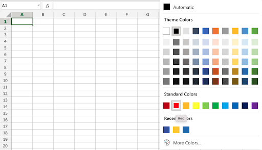
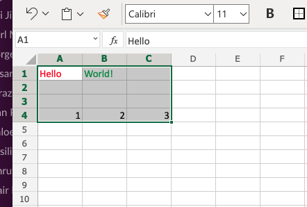
Lets try an example, step by step:
- Select standard font color Red
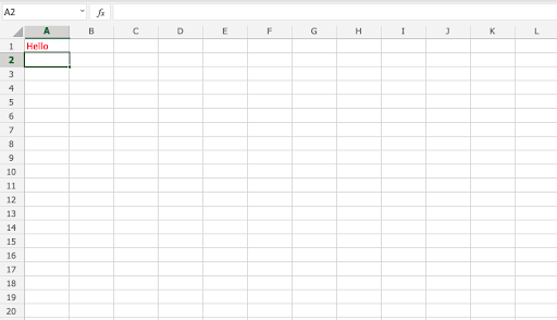
- Type A1(Hello)
- Hit enter
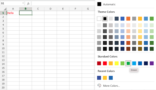
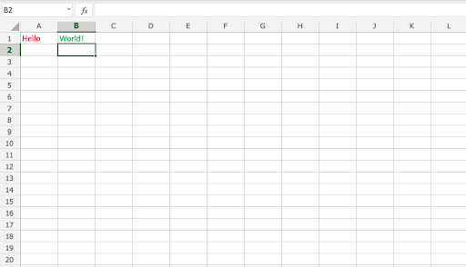
- Select standard font color Green
- Type B1(World!)
- Hit enter
Font Name
The default font in Excel is Calibri.
The font name can be changed for both numbers and text.
Why change the font name in Excel?
- Make the data easier to read
- Make the presentation more appealing
How to change the font name:
- Select a range
- Click the font name drop down menu
- Select a font
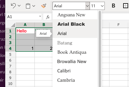
Let’s have a look at an example.
- Select
A1:C4 - Click the font name drop down menu
- Select Arial
The example has both text (A1:B1) and numbers (A4:C4)
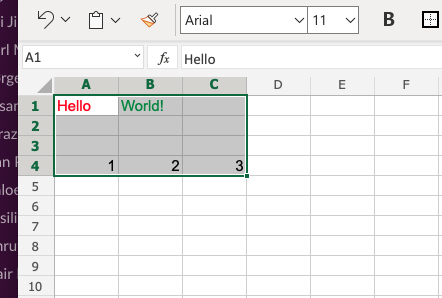
Good job! You have successfully changed the fonts from Calibri to Arial for the range A1:C4.
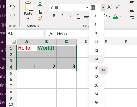
Font Size
To change the font size of the font, just click on the font size drop down menu:
Font Characteristics
You can apply different characteristics to fonts such as:
- Bold
- Italic
- Underlined
- Strike though
The commands can be found below the font name drop down menu:
Bold is applied by either clicking the Bold (B) icon in the Ribbon or using the keyboard shortcut CTRL + B or Command + B
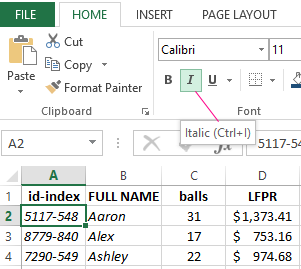
Italic is applied by either clicking the Italic (I) icon or using the keyboard shortcut CTRL + I or Command + I
Underline is applied by either clicking the Underline (U) icon or using the keyboard shortcut CTRL + U or Command + U
Strikethrough is applied by either clicking the Strikethrough (ab) icon or using the keyboard shortcut CTRL + 5 or Command + Shift + X
Chapter Summary
Fonts can be changed in four different ways: color, font name, size and other characteristics. The fonts are changed to make the spreadsheet more readable and delicate.

Changing the appearance of the text in a spreadsheet can make it easier to read. But how do you adjust the font, size and colour of the text? And how do you apply effects? In this article, we provide a quick guide to formatting text in Microsoft Excel.
How to Adjust Fonts in Excel
To change the font used in a cell in Microsoft Excel, you will need to:
- Select all of the cells that you wish to format with the cursor.
- Go to the Home tab on the main ribbon.
- Click the fonts dropdown (i.e. the menu with the name of the current font in it).
- Select the font you want to use from the list.
This will automatically change the typeface for any text already in the selected cell(s), plus any text later typed into the formatted cell(s).
Changing the Font Size in Excel
To change the font size in Microsoft Excel, all you need to do is:
- Select the cell(s) you want to format with the cursor.
- Click the font size dropdown on the Home tab of the ribbon (i.e. the dropdown next to the main font menu).
- Select a value from the list to adjust the size of the text in the selected cell(s).
You can also increase or decrease the font size by one step via the capital ‘A’ buttons with up and down arrows next to this dropdown.
Changing the Font Colour in Excel
To change the font colour in Microsoft Excel:
- Select the cell(s) you want to format.
- Click the font colour button on the Home tab (see below).
- Select a colour from the options available (or click More Colors… at the bottom of this menu to open a new pop-up with custom colours).
You can also change the background colour of a cell by using the Fill Color option to the left of the font colour menu (i.e. the paint bucket icon).
How to Apply Effects in Excel
In Excel, you can also apply italics, bold, and underlining to text. These effects can all be found next to each other in the font group of the Home tab.
Find this useful?
Subscribe to our newsletter and get writing tips from our editors straight to your inbox.
To apply your preferred style(s), select the cell(s) you wish to change, and then click on the B for bold, I for italics or U for underlining.
You also add strikethrough, subscript or superscript to text in Excel.
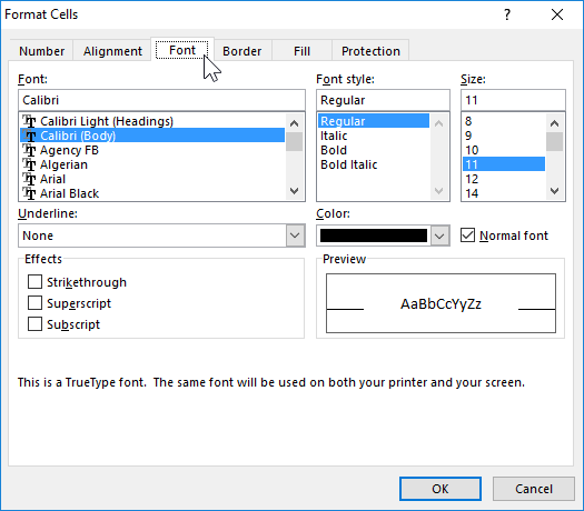
To do this, click the arrow in the bottom right of the font group to open the Format Cells pop-up. Make sure the Font tab is selected, then select your required formatting from the options in the Effects section of the window.
You can make changes to the font, font size and font colour from this pop-up window too, if required, though it is usually quicker to do it via the Home tab.
Formatting Part of a Cell
Finally, what if you want to format a specific part of the text within a cell rather than all the text in a cell? Here’s how you do this:
- Select the cell with the text you want to format.
- In the formula bar, select the specific text you would like to change.
- Choose your preferred formatting using the options set out above.
The change will then be applied in the selected cell, but not in the formula bar.
Expert Spreadsheet Proofreading
Hopefully, this post has explained some of the basics of formatting text in Excel. But you’ll also want the text in your spreadsheets to be error-free. Why not send in a document today and have it checked by our spreadsheet experts?
By default in Excel, the text is on the left side, and the numbers – on the right one. The change in these positions is sometimes justified, but often makes it difficult to distinguish a number from a text.
Treat to the text formatting with moderation. Do not forget, that a stylishly designed document should not contain more than 2 – 3 types of font. There should be no more than 2 – 3 colors, but more shades are allowed.
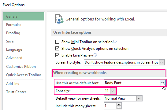
The changing of the default font in Excel
How in Excel to set the default font? For this you need to change 2 parameters in the settings:
- Go to the settings «FILE» – «Options» – «General».
- In the «When creating new workbooks» section, select the required «Font» from the drop-down list.
- Below specify its size and click OK.
The expanding of selected items
To show how to change the default font in Excel, we will format the text in the cells of the data table. The headings of the columns will be highlighted in bold and increase the size of the characters. The text data will be done in italic italics.
The solution of this task is no different from using the tools that Word has. The sequence of actions is as follows:
- Select the range with the column headings of the table.
- On the «HOME» tool tab, press the «B» (bold) button or the CTRL + B key combination.
- In the font size field, we click the mouse and enter our value – is 12, then click «Etner» (you can also specify the font size from the drop-down list of the field). On the same tab, click the «Align Center» button or the hotkey combination: CTRL + E.
- Now select the text data of table A2:B4 and click on the button «Italic» (CTRL + I).
This task can be solved in another way, using the «Format Cells» dialog box. It has more possibilities for formatting text in Excel.
- Again select the range A1 : D1.
- Call the «Format Cells» dialog box using the corner button on the «HOME» tab in the «Align» tool section or press the CTRL + 1 (or CTRL + SHIFT + P) combination. We are interested in the «Font» tab:
- Here we can customize the text in the «Font» tab. In the «Inscription» field, select «Bold Italic». In the Size field, select or set the size to 14.
- Go to the «Alignment» tab.
- In the drop-down list «horizontally», set the value «centered». In the «vertical» list, specify «at the top».
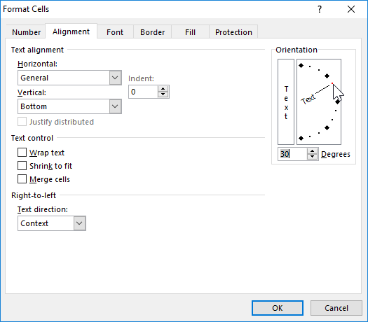
Increase the height of line 1 approximately 2 times. Now you can see that the text of the table headings is centered and is adjacent to the upper edge of the cells.
The formatting the values of the cells helps us to make the data readable and presentable, that are easier to perceive and assimilate. For example, the number 12 can be formatted as 12 $ or 12% or 12 pcs.
In addition, the standard format «General» looks gray and not presentable, but it’s also not too much to overdo it.
In the next lessons of this section, we’ll take a closer look at the possibilities of formatting in Excel.
Transcript
In this lesson we’ll look at how to format cells with a particular font and to change the font size.
Let’s take a look.
Here we have a simple coffee menu. Let’s improve the formatting by applying some custom fonts.
To apply a font to one or more cells, first select the cells you’d like to format. In this case, let’s start by applying a new font to the entire worksheet.
The easiest way to apply a font is to use the menu in the Font group on the home tab of the ribbon. The font menu on the ribbon displays each font in its own typeface. To apply a font, just click a font in the menu.
Let’s also apply the currency format to all prices. Use the Control key to add non-adjacent cells to a selection, then apply the format.
Now, let’s apply a different font to the headings. First, we need to select all the headings using the Control key as before.
The font controls on the ribbon have a nice feature called «live preview.» When you hover your mouse over a font, Excel will display a preview of that font applied to the worksheet. When you move your mouse away, the preview disappears.
This makes it easy to quickly experiment with fonts without actually having to apply them. To leave the font menu without applying a font, just press Escape.
If you know the name of font you’d like to apply, you can speed things up by typing the first few letters of the name in the font menu.
Excel will scroll the list as needed and stop on the best match. To find a different font, just backspace and start typing again. Press Enter to accept the font that has been highlighted in the font menu.
To adjust font size, you have several options. You can select from a list of common sizes from the font size menu, or you can just type a size directly into the list.
Excel also provides buttons to increase and decrease font size. The first button increases font size, and the second button decreases font size.