
Format a date the way you want
Excel for Microsoft 365 Excel for Microsoft 365 for Mac Excel for the web Excel 2021 Excel 2021 for Mac Excel 2019 Excel 2019 for Mac Excel 2016 Excel 2016 for Mac Excel 2013 Excel 2010 Excel 2007 Excel for Mac 2011 More…Less
When you enter some text into a cell such as «2/2″, Excel assumes that this is a date and formats it according to the default date setting in Control Panel. Excel might format it as «2-Feb». If you change your date setting in Control Panel, the default date format in Excel will change accordingly. If you don’t like the default date format, you can choose another date format in Excel, such as «February 2, 2012″ or «2/2/12″. You can also create your own custom format in Excel desktop.
Follow these steps:
-
Select the cells you want to format.
-
Press CTRL+1.
-
In the Format Cells box, click the Number tab.
-
In the Category list, click Date.

-
Under Type, pick a date format. Your format will preview in the Sample box with the first date in your data.
Note: Date formats that begin with an asterisk (*) will change if you change the regional date and time settings in Control Panel. Formats without an asterisk won’t change.
-
If you want to use a date format according to how another language displays dates, choose the language in Locale (location).

Tip: Do you have numbers showing up in your cells as #####? It’s likely that your cell isn’t wide enough to show the whole number. Try double-clicking the right border of the column that contains the cells with #####. This will resize the column to fit the number. You can also drag the right border of the column to make it any size you want.
If you want to use a format that isn’t in the Type box, you can create your own. The easiest way to do this is to start from a format this is close to what you want.
-
Select the cells you want to format.
-
Press CTRL+1.
-
In the Format Cells box, click the Number tab.
-
In the Category list, click Date, and then choose a date format you want in Type. You can adjust this format in the last step below.
-
Go back to the Category list, and choose Custom. Under Type, you’ll see the format code for the date format you chose in the previous step. The built-in date format can’t be changed, so don’t worry about messing it up. The changes you make will only apply to the custom format you’re creating.
-
In the Type box, make the changes you want using code from the table below.
|
To display |
Use this code |
|---|---|
|
Months as 1–12 |
m |
|
Months as 01–12 |
mm |
|
Months as Jan–Dec |
mmm |
|
Months as January–December |
mmmm |
|
Months as the first letter of the month |
mmmmm |
|
Days as 1–31 |
d |
|
Days as 01–31 |
dd |
|
Days as Sun–Sat |
ddd |
|
Days as Sunday–Saturday |
dddd |
|
Years as 00–99 |
yy |
|
Years as 1900–9999 |
yyyy |
If you’re modifying a format that includes time values, and you use «m» immediately after the «h» or «hh» code or immediately before the «ss» code, Excel displays minutes instead of the month.
-
To quickly use the default date format, click the cell with the date, and then press CTRL+SHIFT+#.
-
If a cell displays ##### after you apply date formatting to it, the cell probably isn’t wide enough to show the whole number. Try double-clicking the right border of the column that contains the cells with #####. This will resize the column to fit the number. You can also drag the right border of the column to make it any size you want.
-
To quickly enter the current date in your worksheet, select any empty cell, press CTRL+; (semicolon), and then press ENTER, if necessary.
-
To enter a date that will update to the current date each time you reopen a worksheet or recalculate a formula, type =TODAY() in an empty cell, and then press ENTER.
When you enter some text into a cell such as «2/2″, Excel assumes that this is a date and formats it according to the default date setting in Control Panel. Excel might format it as «2-Feb». If you change your date setting in Control Panel, the default date format in Excel will change accordingly. If you don’t like the default date format, you can choose another date format in Excel, such as «February 2, 2012″ or «2/2/12″. You can also create your own custom format in Excel desktop.
Follow these steps:
-
Select the cells you want to format.
-
Press Control+1 or Command+1.
-
In the Format Cells box, click the Number tab.
-
In the Category list, click Date.
-
Under Type, pick a date format. Your format will preview in the Sample box with the first date in your data.
Note: Date formats that begin with an asterisk (*) will change if you change the regional date and time settings in Control Panel. Formats without an asterisk won’t change.
-
If you want to use a date format according to how another language displays dates, choose the language in Locale (location).
Tip: Do you have numbers showing up in your cells as #####? It’s likely that your cell isn’t wide enough to show the whole number. Try double-clicking the right border of the column that contains the cells with #####. This will resize the column to fit the number. You can also drag the right border of the column to make it any size you want.
If you want to use a format that isn’t in the Type box, you can create your own. The easiest way to do this is to start from a format this is close to what you want.
-
Select the cells you want to format.
-
Press Control+1 or Command+1.
-
In the Format Cells box, click the Number tab.
-
In the Category list, click Date, and then choose a date format you want in Type. You can adjust this format in the last step below.
-
Go back to the Category list, and choose Custom. Under Type, you’ll see the format code for the date format you chose in the previous step. The built-in date format can’t be changed, so don’t worry about messing it up. The changes you make will only apply to the custom format you’re creating.
-
In the Type box, make the changes you want using code from the table below.
|
To display |
Use this code |
|---|---|
|
Months as 1–12 |
m |
|
Months as 01–12 |
mm |
|
Months as Jan–Dec |
mmm |
|
Months as January–December |
mmmm |
|
Months as the first letter of the month |
mmmmm |
|
Days as 1–31 |
d |
|
Days as 01–31 |
dd |
|
Days as Sun–Sat |
ddd |
|
Days as Sunday–Saturday |
dddd |
|
Years as 00–99 |
yy |
|
Years as 1900–9999 |
yyyy |
If you’re modifying a format that includes time values, and you use «m» immediately after the «h» or «hh» code or immediately before the «ss» code, Excel displays minutes instead of the month.
-
To quickly use the default date format, click the cell with the date, and then press CTRL+SHIFT+#.
-
If a cell displays ##### after you apply date formatting to it, the cell probably isn’t wide enough to show the whole number. Try double-clicking the right border of the column that contains the cells with #####. This will resize the column to fit the number. You can also drag the right border of the column to make it any size you want.
-
To quickly enter the current date in your worksheet, select any empty cell, press CTRL+; (semicolon), and then press ENTER, if necessary.
-
To enter a date that will update to the current date each time you reopen a worksheet or recalculate a formula, type =TODAY() in an empty cell, and then press ENTER.
When you type something like 2/2 in a cell, Excel for the web thinks you’re typing a date and shows it as 2-Feb. But you can change the date to be shorter or longer.
To see a short date like 2/2/2013, select the cell, and then click Home > Number Format > Short Date. For a longer date like Saturday, February 02, 2013, pick Long Date instead.
-
If a cell displays ##### after you apply date formatting to it, the cell probably isn’t wide enough to show the whole number. Try dragging the column that contains the cells with #####. This will resize the column to fit the number.
-
To enter a date that will update to the current date each time you reopen a worksheet or recalculate a formula, type =TODAY() in an empty cell, and then press ENTER.
Need more help?
You can always ask an expert in the Excel Tech Community or get support in the Answers community.
Need more help?
Want more options?
Explore subscription benefits, browse training courses, learn how to secure your device, and more.
Communities help you ask and answer questions, give feedback, and hear from experts with rich knowledge.
In this guide, we’ll learn how to change date format in Excel. Date and Time data is an integral part of any statistical document or sheet. It is important to accurately track and analyze events, sales, figures, and others.
By convention, Excel uses a general data format that may be as per your need. But in most cases, that format may need to be customized.
Changing the format of Date in a particular cell or all the cells in your Excel sheet is an easy process and doesn’t require any complex methodologies. Excel provides a wide range of formatting options based on Location and Languages which helps in better date formatting in native language and style. Also, For some Languages there is also features to select from different Calendar types.
Follow the below step-by-step tutorial to change date format in Excel quickly and easily.
Step 1. Select the range of cells containing the date
To start with, select the cell values where want to change the date format, as shown in the image below.

Step 2. Go to Number Format dropdown
- To select ‘Number Format’, go to ‘Home‘ in the option menu and look for Number Format, as shown below
- Then from the drop-down menu, select ‘More Number Formats‘ to reveal the ‘Number Format’ dialogue menu.

- Alternatively, you may directly go to Number Format, by right-clicking on the selected cell/s
- Click on ‘Number Format’.

Step 3. Choose Date
- From the Category menu on the right, choose ‘Date‘.

Now, to apply any date formatting type, select it from the right panel of the pop-up menu of Number Format. Click on ‘OK‘ to apply the formatting to the selected cell/s.
Note: You may check the date format implementation in the ‘Sample‘ at the top of the menu option
Choose the Date Type
The general option type to choose from a variety of Date Formatting options. Scroll down in this section to reveal a plethora of options for formatting, ranging from date, text (month name), year, and others.
This option can be perceived as the display menu, as the formatting options in this will keep on changing as per the selection in Locale(Location) and Calendar type.

Choose the Locale (location)
This option features the Location or Language options to help format the date accordingly. This option is probably the most used option as users require to format the date according to their or audience preference as per the native formatting style, based on language and location.
Choose any language or Location from this options menu. After selecting, all the supported date format options available for that particular locale will be available for selecting in the above Type menu.

Choose the type of calendar
This option reveals different calendar types available based on the Locale(Location) selected from the above option menu. This formatting option is only available for certain Locale and not all.
As shown in our example below, the variety of calendar types available for selection are only available for the Locale (location) selected (here, Arabia), for other locales the calendar type might be different or not at all present.

To apply selected formatting, you will need to click ‘OK‘ after selection to apply to your dates.
Conclusion
That’s It! You can now easily convert your dates to your desired format style easily.
We hope you learned and enjoyed this lesson and we’ll be back soon with another awesome Excel tutorial at QuickExcel!
Even though dates and time are actually stored as a regular number known as the date serial number, we can make use of extensive Excel date and time formatting options to display them just the way we want.
We can access some quick date and time formats from the Home tab > in the Number group:
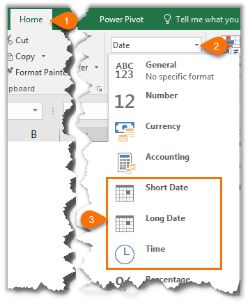
We can also create our own custom date and time formats to suit our needs. Let’s take a look.
- Select the cell(s) containing the dates you want to format.
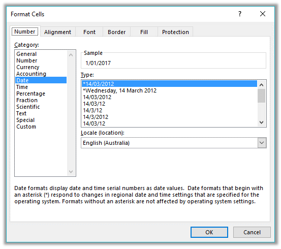
- Press CTRL+1, or right-click > Format Cells to open the Format Cells dialog box.
- On the Number tab select ‘Date’ in the Categories list. This brings up a list of default date formats you can select from in the ‘Type’ list. Likewise for the Time category.
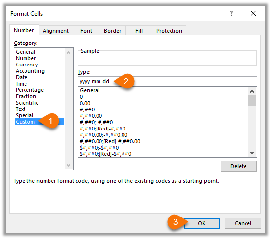
We aren’t limited to the defaults though. You can create your own Custom date or time formats in the ‘Custom’ category. These custom formats are saved for you to re-use in the current file.
Custom Date Formatting Characters
Excel recognises the following characters and sets of characters for date formatting.
| Character | Explanation | Date | Formatted | |
| d | Displays the day as a number without a leading zero. | 3/09/2016 | 3 | |
| dd | Displays the day as a number with a leading zero when appropriate. | 3/09/2016 | 03 | |
| ddd | Displays the day as an abbreviation (Sun to Sat). | 3/09/2016 | Sat | |
| dddd | Displays the day as a full name (Sunday to Saturday). | 3/09/2016 | Saturday | |
| m | Displays the month as a number without a leading zero. | 3/09/2016 | 9 | |
| mm | Displays the month as a number with a leading zero when appropriate. | 3/09/2016 | 09 | |
| mmm | Displays the month as an abbreviation (Jan to Dec). | 3/09/2016 | Sep | |
| mmmm | Displays the month as a full name (January to December). | 3/09/2016 | September | |
| mmmmm | Displays the month as a single letter (J to D). | 3/09/2016 | S | |
| yy | Displays the year as a two-digit number. | 3/09/2016 | 16 | |
| yyyy | Displays the year as a four-digit number. | 3/09/2016 | 2016 |
Custom Date Formatting Examples
We can bring the characters together to create our own custom formats. Some examples below:
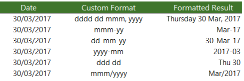
Remember; the custom format doesn’t alter the underlying date serial number, it is still the same.
Custom Time Formatting Characters
Like dates, time also has its own set of custom formatting characters, as listed below:
| Character | Explanation | ||
| h | Displays the hour as a number without a leading zero. | ||
| [h] | Displays elapsed time in hours. If you are working with a formula that returns a time in which the number of hours exceeds 24, use a number format that resembles [h]:mm:ss or [h]:mm | ||
| hh | Displays the hour as a number with a leading zero when appropriate. If the format contains AM or PM, the hour is based on the 12-hour clock. Otherwise, the hour is based on the 24-hour clock. | ||
| m | Displays the minute as a number without a leading zero.* | ||
| [m] | Displays elapsed time in minutes. If you are working with a formula that returns a time in which the number of minutes exceeds 60, use a number format that resembles [mm]:ss. | ||
| mm | Displays the minute as a number with a leading zero when appropriate.* | ||
| s | Displays the second as a number without a leading zero. | ||
| [s] | Displays elapsed time in seconds. If you are working with a formula that returns a time in which the number of seconds exceeds 60, use a number format that resembles [ss]. | ||
| ss | Displays the second as a number with a leading zero when appropriate. If you want to display fractions of a second, use a number format that resembles h:mm:ss.00. | ||
| AM/PM, am/pm, A/P, a/p | Displays the hour using a 12-hour clock. Excel displays AM, am, A, or a for times from midnight until noon and PM, pm, P, or p for times from noon until midnight. |
*Note: The m or mm code must appear immediately after the h or hh code or immediately before the ss code; otherwise, Excel displays the month instead of minutes.
Custom Time Formatting Examples
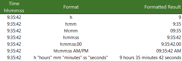
Note: if your PC region settings have the Date & Time formats set to show the Short Time as hh:mm tt or the Long Time as hh:mm:ss tt then this may override any single ‘h’ formats and display them as ‘hh’.
The screenshot above is what I see with my PC region settings for the Short Time as h:mm tt. If you see something different when using a single ‘h’ format, then it will be down to your PC region settings.
More Excel Formatting
Custom cell formatting isn’t limited to dates and times. There is a plethora of formatting options for all types of numbers that we can use to get our reports looking just the way we want. Click here for our comprehensive guide to Excel custom number formatting.
Free eBook — Working with Date & Time in Excel
Everything you need to know about Date and Time in Excel — Download the free eBook and Excel file with detailed instructions.
Enter your email address below to download the comprehensive Excel workbook and PDF.
By submitting your email address you agree that we can email you our Excel newsletter.
So I’ve been battling with this issue all day.
Basically I have it now sorted and part of the solution was a code that Excel itself generated which is:
[$-en-AU]yyyy-mm-dd hh:mm
So, in the first instance,
- in a new spreadsheet, type your entry in as per usual, eg:
2026-01-31 10:00 - set the format of the cell to «custom» and use the above formula, ie
[$-en-AU]yyyy-mm-dd hh:mm - Hit enter and Bob’s your uncle!
Then save it as a CSV file, then close it and re-open it to check Excel hasn’t changed the date format.
The weird thing is if it does work (and I’ve re-tried it a few times successfully), when you check the format of the cell you’ve created, it’s changed the format to «General».
But seriously who cares. As long as it works!!
You can then copy and paste the cell and use it wherever you want!!
I hope this solution works for you!!
Regards
Richard
When you enter a date into Microsoft Excel, the program will format it according to the default date settings. For example, if you want to enter the date February 6, 2020, the date could appear as 6-Feb, February 6, 2020, 6 February, or 02/06/2020, all depending on your settings. You may find that if you change a cell’s formatting to “Standard,” your date becomes stored as integers. For example, February 6, 2020 would become 43865, because Excel bases date formatting off of January 1, 1900. Each of these options are ways to format dates in Excel. To help with organizing data in Excel, learn about how to change the date format in Excel.
Choosing from the Date Format List
Formatting dates in Excel is easiest with the date formats list. Most date formats you may want to use can be found in this menu.
How to Change The Excel Date Format
- Select the cells you want to format
- Click Ctrl+1 or Command+1
- Select the “Numbers” tab
- From the categories, choose “Date”
- From the “Type” menu, select the date format you want

Creating a Custom Excel Date Format Option
To customize the date format, follow the steps for choosing an option from the date format list. Once you’ve selected the closest date format to what you want, you can customize it and change it.
- In the “Category” menu, select “Custom”
- The type you chose earlier will appear. The changes you make will only apply to your customized setting, not to the default
- In the “Type” box, enter the correct code to alter the date
- If you are trying to change the date display to DD/MM/YYYY, simply go to Format Cells > Custom
- Next, Enter DD/MM/YYYY in the available space given.

Converting Date Formats to Other Locales
If you are using dates for several different locations, you might need to convert to a different locale:
- Select the right cell or cells
- Hit Ctrl+1 or Command+1
- From the “Numbers” menu, select “Date”
- Underneath the “Type” menu, there’s a drop-down menu for “Locale”
- Select the right “Locale”

You can also customize the locale settings:
- Follow the steps for customizing a date
- Once you’ve created the right date format, you need to add the locale code to the front of the customized date format
- Choose the right locale codes. All locale codes are formatted as [$-###]. Some examples include:
- [$-409]—English, United States
- [$-804]—Chinese, China
- [$-807]—German, Switzerland
- Find more locale codes

Tips for Displaying Dates in Excel
Once you have the right date format, there are additional tips to help you figure out how to organize data in Excel for your datasets.
- Make sure the cell is wide enough to fit the entire date. If the cell isn’t wide enough, it will display #####. Double click on the right border of the column to make your column expand enough to display the date correctly.
- Change the date system if negative numbers appear as dates. Sometimes Excel will format any negative numbers as a date because of the hyphens. To fix this, select the cells, open the options menu, and select “Advanced.” On that menu, select “Use 1904 date system.”
- Use functions to work with today’s date. If you want a cell to always display the current date, use the formula =TODAY() and press ENTER.
- Convert imported text to dates. If you import from an external database, Excel will automatically register the dates as text. The display may look the same as if they were formatted as dates, but Excel will treat the two differently. You can use the DATEVALUE function to convert.
Why Your Date Format May Not Be Having Issues Changing
There are many reasons why you might be experiencing issues changing the date format in Excel. Listed are a few common difficulties.
- There could be text in the column, not dates (which are actually numbers).
- Dates are left-aligned
- An apostrophe could be included in the date
- A cell may be too wide.
- Negative numbers are formatted as dates
- Excel TEXT function is not being utilized.
Even with correctly formatted dates and displays, organizing data in Excel can only work as well as the data does. Messy data won’t lead to insights during analysis, however, it’s formatted.
Data Preparation with Excel
Formatting data, by doing things like formatting dates, is part of a larger process known as “data preparation,” or all of the steps required to clean, standardize, and prepare data for analytic use.
While data preparation is certainly possible in Excel, it becomes exponentially more difficult as analysts work with larger and more complex datasets. Instead, many of today’s analysts are investing in modern data preparation platforms like Designer Cloud to accelerate the overall data preparation process for data big or small.
Schedule a demo of Designer Cloud to see how it can improve your data preparation process, or try the platform for yourself by getting started with Designer Cloud today.