
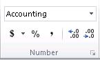
If you want to display numbers as monetary values, you must format those numbers as currency. To do this, you apply either the Currency or Accounting number format to the cells that you want to format. The number formatting options are available on the Home tab, in the Number group.

In this article
-
Format numbers as currency
-
Remove currency formatting
-
What’s the difference between the Currency and Accounting formats?
-
Create a workbook template with specific currency formatting settings
Format numbers as currency
You can display a number with the default currency symbol by selecting the cell or range of cells, and then clicking Accounting Number Format  in the Number group on the Home tab. (If you want to apply the Currency format instead, select the cells, and press Ctrl+Shift+$.)
If you want more control over either format, or you want to change other aspects of formatting for your selection, you can follow these steps.
Select the cells you want to format
On the Home tab, click the Dialog Box Launcher next to Number.

Tip: You can also press Ctrl+1 to open the Format Cells dialog box.
In the Format Cells dialog box, in the Category list, click Currency or Accounting.

In the Symbol box, click the currency symbol that you want.
Note: If you want to display a monetary value without a currency symbol, you can click None.
In the Decimal places box, enter the number of decimal places that you want for the number. For example, to display $138,691 instead of $138,690.63 in the cell, enter 0 in the Decimal places box.
As you make changes, watch the number in the Sample box. It shows you how changing the decimal places will affect the display of a number.
In the Negative numbers box, select the display style you want to use for negative numbers. If you don’t want the existing options for displaying negative numbers, you can create your own number format. For more information about creating custom formats, see Create or delete a custom number format.
Note: The Negative numbers box is not available for the Accounting number format. That’s because it is standard accounting practice to show negative numbers in parentheses.
To close the Format Cells dialog box, click OK.
If Excel displays ##### in a cell after you apply currency formatting to your data, the cell probably isn’t wide enough to display the data. To expand the column width, double-click the right boundary of the column that contains the cells with the ##### error. This automatically resizes the column to fit the number. You can also drag the right boundary until the columns are the size that you want.
Top of Page
Remove currency formatting
If you want to remove the currency formatting, you can follow these steps to reset the number format.
-
Select the cells that have currency formatting.
-
On the Home tab, in the Number group, click General.
Cells that are formatted with the General format do not have a specific number format.
Top of Page
What’s the difference between the Currency and Accounting formats?
Both the Currency and Accounting formats are used to display monetary values. The difference between the two formats is explained in the following table.
|
Format |
Description |
Example |
|
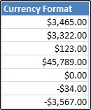
Currency |
When you apply the Currency format to a number, the currency symbol appears right next to the first digit in the cell. You can specify the number of decimal places that you want to use, whether you want to use a thousands separator, and how you want to display negative numbers. Tip: To quickly apply the Currency format, select the cell or range of cells that you want to format, and then press Ctrl+Shift+$. |
|
|
Format |
Description |
Example |
|
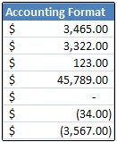
Accounting |
Like the Currency format, the Accounting format is used for monetary values. But, this format aligns the currency symbols and decimal points of numbers in a column. In addition, the Accounting format displays zeros as dashes and negative numbers in parentheses. Like the Currency format, you can specify how many decimal places you want and whether to use a thousands separator. You can’t change the default display of negative numbers unless you create a custom number format. Tip: To quickly apply the Accounting format, select the cell or range of cells that you want to format. On the Home tab, in the Number group, click Accounting Number Format |
|
Top of Page
Create a workbook template with specific currency formatting settings
If you often use currency formatting in your workbooks, you can save time by creating a workbook that includes specific currency formatting settings, and then saving that workbook as a template. You can then use this template to create other workbooks.
-
Create a workbook.
-
Select the worksheet or worksheets for which you want to change the default number formatting.
How to select worksheets
To select
Do this
A single sheet
Click the sheet tab.

If you don’t see the tab that you want, click the tab scrolling buttons to display the tab, and then click the tab.
Two or more adjacent sheets
Click the tab for the first sheet. Then hold down Shift while you click the tab for the last sheet that you want to select.
Two or more nonadjacent sheets
Click the tab for the first sheet. Then hold down Ctrl while you click the tabs of the other sheets that you want to select.
All sheets in a workbook
Right-click a sheet tab, and then click Select All Sheets on the shortcut menu.
Tip When multiple worksheets are selected, [Group] appears in the title bar at the top of the worksheet. To cancel a selection of multiple worksheets in a workbook, click any unselected worksheet. If no unselected sheet is visible, right-click the tab of a selected sheet, and then click Ungroup Sheets.
-
Select the specific cells or columns you want to format, and then apply currency formatting to them.


Make any other customizations that you like to the workbook, and then do the following to save it as a template:
Save the workbook as a template
-
If you’re saving a workbook to a template for the first time, start by setting the default personal templates location:
-
Click File, and then click Options.
-
Click Save, and then under Save workbooks, enter the path to the personal templates location in the Default personal templates location box.
This path is typically: C:UsersPublic DocumentsMy Templates.
-
Click OK.
Once this option is set, all custom templates you save to the My Templates folder automatically appear under Personal on the New page (File > New).
-
-
Click File, and then click Export.
-
Under Export, click Change File Type.
-
In the Workbook File Types box, double-click Template.
-
In the File name box, type the name you want to use for the template.
-
Click Save, and then close the template.

Create a workbook based on the template
-
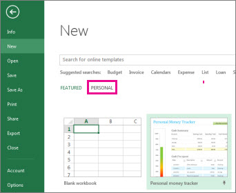
Click File, and then click New.
-
Click Personal.
-
Double-click the template you just created.
Excel creates a new workbook that is based on your template.
Top of Page

In this article, we will learn How to Quickly apply Currency number format in Excel.
Scenario:
To get the currency format Go to Home tab and find a dollar symbol, click it to get currency format. This is too easy then just use keyboard shortcut Ctrl + Shift + 4 ($). format the selected range of cells as u.s. Currency accessing the currency formats in excel as explained below.
Different Currency formats in Excel
There are some recommended currency formats given in the drop down list of currency’s list in Excel.

There popular ones are
- English (India) : Indian currency
- English (United kingdom) : UK dollar
- Euro : European currency
- English (United States) : US dollar
Example :
All of these might be confusing to understand. Let’s understand how to use the function using an example. Here we have two numbers, one positive and one negative. See what happens when we select both numbers and use Ctrl + Shift + $ (from keyboard).

As you can see the transformation to $ (dollar) currency. You can get a different currency format using the Format cells option (shortcut key Ctrl + 1).
More shortcut keys
| Format | Shortcut key |
| General number | Ctrl + Shift + ~ |
| Currency format | Ctrl + Shift + $ |
| Percentage format | Ctrl + Shift + % |
| Scientific format | Ctrl + Shift + ^ |
| Date format | Ctrl + Shift + # |
| Time format | Ctrl + Shift + @ |
| Custom formats | Ctrl + 1 |
Here are all the observational notes using the formula in Excel
Notes :
- Currency format use negative values in red and bracket depending on the selected currency.
- Use number formatting to convert the value into another format. The value remains the same.
- Use percentage format when using percentage rate values in Excel.
- Every Excel Formula starts with ( = ) sign.
- Numerical values can be given directly or using the cell reference.
Hope this article about How to Quickly apply Currency number format in Excel is explanatory. Find more articles on calculating values and related Excel formulas here. If you liked our blogs, share it with your friends on Facebook. And also you can follow us on Twitter and Facebook. We would love to hear from you, do let us know how we can improve, complement or innovate our work and make it better for you. Write to us at info@exceltip.com.
Related Articles :
How to Convert Number to Words in Excel in Rupees : Excel does not provide any function that converts a number or amount in words in Indian rupees or any currency. Create a custom Excel formula to convert numbers to words in Indian rupees using the VBA code given in the link.
How to Insert Row using Shortcut in Excel : These shortcuts will help you insert single and multiple rows quickly. Learn more about shortcuts by clicking the link.
Excel Shortcut Keys for Merge and Center : This Merge and Center shortcut helps you quickly merge and unmerge cells. Learn more about shortcuts by clicking the link.
Paste Special Shortcut in Mac and Windows : In windows, the keyboard shortcut for paste special is Ctrl + Alt + V. Whereas in Mac, use Ctrl + COMMAND + V key combination to open the paste special dialog in Excel.
How to Select Entire Column and Row Using Keyboard Shortcuts in Excel : Selecting cells is a very common function in Excel. Use Ctrl + Space to select columns and Shift + Space to select rows in Excel.
How to use Shortcut Keys for Sort & filter in Excel : Use Ctrl + Shift + L from keyboard to apply sort and filter on table in Excel.
Popular Articles :
50 Excel Shortcuts to Increase Your Productivity : Get faster at your tasks in Excel. These shortcuts will help you increase your work efficiency in Excel.
How to use the VLOOKUP Function in Excel : This is one of the most used and popular functions of excel that is used to lookup value from different ranges and sheets.
How to use the IF Function in Excel : The IF statement in Excel checks the condition and returns a specific value if the condition is TRUE or returns another specific value if FALSE.
How to use the SUMIF Function in Excel : This is another dashboard essential function. This helps you sum up values on specific conditions.
How to use the COUNTIF Function in Excel : Count values with conditions using this amazing function. You don’t need to filter your data to count specific values. Countif function is essential to prepare your dashboard.
Transcript
In this lesson we’ll take a look at the Currency format. The Currency format is designed to display a currency symbol along with numbers. It has options for the currency symbol itself, the number of decimal places, and negative number handling.
Let’s take a look.
Let’s start off by copying a set of numbers in General format across our table, and then apply the default currency format to the columns C through H.
Now let’s select cells in column D and check the options available for currency in the Format Cells dialog box. Like Number format, the Currency format provides options for decimal places and handling negative numbers. However, it does not provide an option for a thousandths separator—this is always enabled for Currency.
Let’s set decimal places to zero, and close the dialog. Like Number format, we can also adjust decimal places up and down using the buttons on the ribbon.
To display negative numbers in parentheses, we need to visit the Format Cells dialog box again.
With parentheses enabled, Excel shifts all numbers a bit to the left to keep numbers aligned on the decimal point.
We’ll need to head to the Format Cells dialog box again to change the currency symbol to the British Pound. Excel provides a huge list of options for currency symbols, including abbreviations.
Note that there are shortcuts on the ribbon that include a currency symbol, but these actually apply the Accounting number format, which may not be desired.
You can use the Format Cells dialog to switch from Accounting back to Currency, leaving the Euro symbol intact.
One more visit to the Format Cells dialog to select the currency symbol of None.
Note that selecting None as the currency symbol has an interesting result: the format of the cells in column H is now no longer Currency, but is simply Number.
Download PC Repair Tool to quickly find & fix Windows errors automatically
Microsoft Office Excel can be configured to display a number with the default currency symbol. In addition to the options for currency symbols, the format has options for the number of decimal places and negative number handling too. The case in point here is how you add a currency symbol before a number in the cells since simply typing a symbol sign at the beginning of a currency value will not be recognized as a number. Let’s see how to do it.

Excel users wanting to display numbers as monetary values, must first format those numbers as currency.
To do this, apply either the Currency or Accounting number format to the cells that you want to format. The number formatting options are visible under the Home tab of the ribbon menu, in the Number group.

Next, for displaying a number with the default currency symbol adjacent to it, select the cell or range of cells, and then click Accounting Number Format Button image in the Number group on the Home tab. (If you want to apply the Currency format instead, select the cells, and press Ctrl+Shift+$.)
If you would like to change other aspects of formatting for your selection,
Select the cells you would want to format.
Next, on the Home tab, click the Dialog Box Launcher adjacent to Number. See the screenshot below.
Then, in the Format Cells dialog box, in the Category list, click Currency or Accounting.

Thereafter, under the Symbol box, click the currency symbol that you want. If you do not wish to display a monetary value, simply choose the None option. If required, enter the number of decimal places that you want for the number.
As you make changes, it will reflect in the number in the Sample box, indicating changing the decimal places affect the display of a number.
Now read: How to perform calculations with Range Calculations app for Excel.

A post-graduate in Biotechnology, Hemant switched gears to writing about Microsoft technologies and has been a contributor to TheWindowsClub since then. When he is not working, you can usually find him out traveling to different places or indulging himself in binge-watching.
When you type numbers into a cell in Excel Online, that data is going to be formatted as a number by default. This means that there won’t be any decimal places unless you manually add them. This can create a problem when you are working with currency values, however, as the inconsistency with the amount of decimal places can make it difficult to read the information.
Fortunately Excel Online lets you format your data so that it is of the appropriate type for the data that you’ve entered, and there are some currency formats that you can achieve to meet this goal. Our tutorial below will show you how to select some cells in your Excel Online spreadsheet and format them as currency.
How to Format Data as Currency in Excel Online
The steps in this article were performed in the desktop version of Google Chrome, but will also work in other desktop Web browsers like Firefox or Microsoft Edge. Note that you can format your currency data to either show or hide the currency symbol next to the data value.
Step 1: Sign into Excel Online at https://office.live.com/start/Excel.aspx and sign into the Microsoft account containing the Excel file with data that you wish to format as currency.
Step 2: Open the Excel file.
Step 3: Select the cells containing the data to format as currency. Note that you can select an entire row or column by clicking the row number or column letter at the left or top of that row or column, respectively.
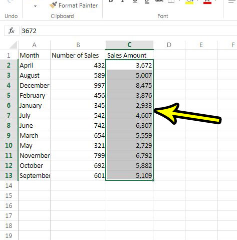
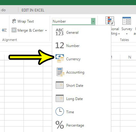
Step 4: Click the dropdown menu at the top of the Number section of the ribbon.
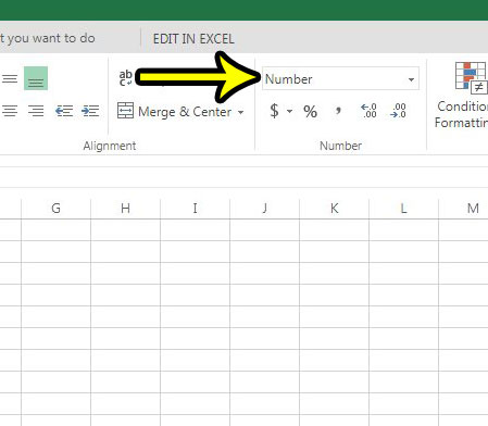
Step 5: Choose the Currency option from the list.
If you would prefer to hide the currency symbol, then right-click the selected cells and choose the Number Format option.
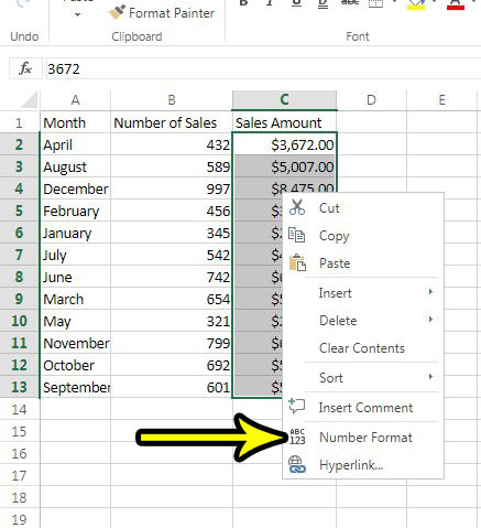
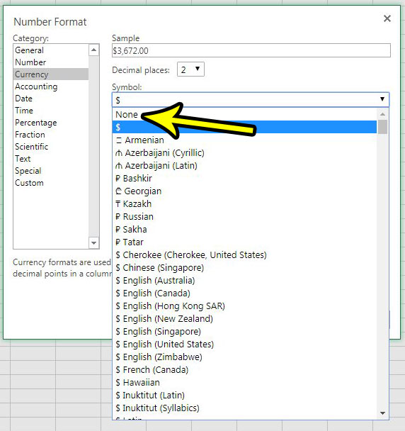
You can then click the Symbol dropdown menu and choose the None option, then click the OK button at the bottom of the window to apply the change.
For more information on changing cell formatting in Excel Online, check out this article. There are a number of different formatting options that can help you get your data to display the way that you need.

Kermit Matthews is a freelance writer based in Philadelphia, Pennsylvania with more than a decade of experience writing technology guides. He has a Bachelor’s and Master’s degree in Computer Science and has spent much of his professional career in IT management.
He specializes in writing content about iPhones, Android devices, Microsoft Office, and many other popular applications and devices.
Read his full bio here.