Формат ячеек excel миф

Formatting Numbers in Excel VBA

Numbers come in all kinds of formats in Excel worksheets. You may already be familiar with the pop-up window in Excel for making use of different numerical formats:

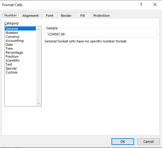
Formatting of numbers make the numbers easier to read and understand. The Excel default for numbers entered into cells is ‘General’ format, which means that the number is displayed exactly as you typed it in.

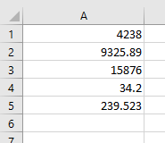
For example, if you enter a round number e.g. 4238, it will be displayed as 4238 with no decimal point or thousands separators. A decimal number such as 9325.89 will be displayed with the decimal point and the decimals. This means that it will not line up in the column with the round numbers, and will look extremely messy.

Also, without showing the thousands separators, it is difficult to see how large a number actually is without counting the individual digits.  Is it in millions or tens of millions?

From the point of view of a user looking down a column of numbers, this makes it quite difficult to read and compare.

In VBA you have access to exactly the same range of formats that you have on the front end of Excel. This applies to not only an entered value in a cell on a worksheet, but also things like message boxes, UserForm controls, charts and graphs, and the Excel status bar at the bottom left hand corner of the worksheet.

The Format function is an extremely useful function in VBA in presentation terms, but it is also very complex in terms of the flexibility offered in how numbers are displayed.

How to Use the Format Function in VBA

If you are showing a message box, then the Format function can be used directly:

MsgBox Format(1234567.89, "#,##0.00")

This will display a large number using commas to separate the thousands and to show 2 decimal places.  The result will be 1,234,567.89.  The zeros in place of the hash ensure that decimals will be shown as 00 in whole numbers, and that there is a leading zero for a number which is less than 1

The hashtag symbol (#) represents a digit placeholder which displays a digit if it is available in that position, or else nothing.

You can also use the format function to address an individual cell, or a range of cells to change the format:

Sheets("Sheet1").Range("A1:A10").NumberFormat = "#,##0.00"

This code will set the range of cells (A1 to A10) to a custom format which separates the thousands with commas and shows 2 decimal places.

If you check the format of the cells on the Excel front end, you will find that a new custom format has been created.

You can also format numbers on the Excel Status Bar at the bottom left hand corner of the Excel window:

Application.StatusBar = Format(1234567.89, "#,##0.00")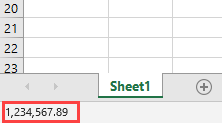

You clear this from the status bar by using:

Application.StatusBar = ""

Creating a Format String

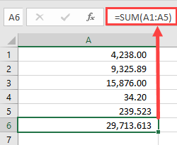
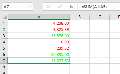
This example will add the text ‘Total Sales’ after each number, as well as including a thousands separator

Sheets("Sheet1").Range("A1:A6").NumberFormat = "#,##0.00"" Total Sales"""

This is what your numbers will look like:

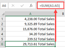
Note that cell A6 has a ‘SUM’ formula, and this will include the ‘Total Sales’ text without requiring formatting.  If the formatting is applied, as in the above code, it will not put an extra instance of ‘Total Sales’ into cell A6

Although the cells now display alpha numeric characters, the numbers are still present in numeric form. The ‘SUM’ formula still works because it is using the numeric value in the background, not how the number is formatted.

The comma in the format string provides the thousands separator. Note that you only need to put this in the string once.  If the number runs into millions or billions, it will still separate the digits into groups of 3

The zero in the format string (0) is a digit placeholder. It displays a digit if it is there, or a zero. Its positioning is very important to ensure uniformity with the formatting

In the format string, the hash characters (#) will display nothing if there is no digit.  However, if there is a number like .8 (all decimals), we want it to show as 0.80 so that it lines up with the other numbers.

By using a single zero to the left of the decimal point and two zeros to the right of the decimal point in the format string, this will give the required result (0.80).

If there was only one zero to the right of the decimal point, then the result would be ‘0.8’ and everything would be displayed to one decimal place.

Using a Format String for Alignment

We may want to see all the decimal numbers in a range aligned on their decimal points, so that all the decimal points are directly under each other, however many places of decimals there are on each number.

You can use a question mark (?) within your format string to do this.  The ‘?’ indicates that a number is shown if it is available, or a space

Sheets("Sheet1").Range("A1:A6").NumberFormat = "#,##0.00??"

This will display your numbers as follows:

All the decimal points now line up underneath each other.  Cell A5 has three decimal places and this would throw the alignment out normally, but using the ‘?’ character aligns everything perfectly.

Using Literal Characters Within the Format String

You can add any literal character into your format string by preceding it with a backslash ().

Suppose that you want to show a particular currency indicator for your numbers which is not based on your locale.  The problem is that if you use a currency indicator, Excel automatically refers to your local and changes it to the one appropriate for the locale that is set on the Windows Control Panel.  This could have implications if your Excel application is being distributed in other countries and you want to ensure that whatever the locale is, the currency indicator is always the same.

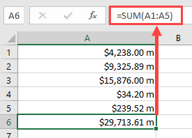
You may also want to indicate that the numbers are in millions in the following example:

Sheets("Sheet1").Range("A1:A6").NumberFormat = "$#,##0.00 m"

This will produce the following results on your worksheet:

In using a backslash to display literal characters, you do not need to use a backslash for each individual character within a string. You can use:

Sheets("Sheet1").Range("A1:A6").NumberFormat = "$#,##0.00 mill"

This will display ‘mill’ after every number within the formatted range.

You can use most characters as literals, but not reserved characters such as 0, #,?

Use of Commas in a Format String

We have already seen that commas can be used to create thousands separators for large numbers, but they can also be used in another way.

By using them at the end of the numeric part of the format string, they act as scalers of thousands. In other words, they will divide each number by 1,000 every time there is a comma.

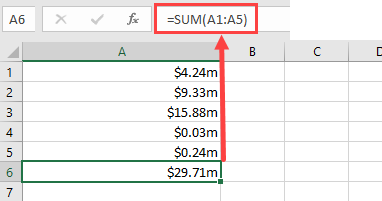
In the example data, we are showing it with an indicator that it is in millions. By inserting one comma into the format string, we can show those numbers divided by 1,000.

Sheets("Sheet1").Range("A1:A6").NumberFormat = "$#,##0.00,m"

This will show the numbers divided by 1,000 although the original number will still be in background in the cell.

If you put two commas in the format string, then the numbers will be divided by a million

Sheets("Sheet1").Range("A1:A6").NumberFormat = "$#,##0.00,,m"

This will be the result using only one comma (divide by 1,000):

VBA Coding Made Easy

Stop searching for VBA code online. Learn more about AutoMacro — A VBA Code Builder that allows beginners to code procedures from scratch with minimal coding knowledge and with many time-saving features for all users!

Learn More

Creating Conditional Formatting within the Format String

You could set up conditional formatting on the front end of Excel, but you can also do it within your VBA code, which means that you can manipulate the format string programmatically to make changes.

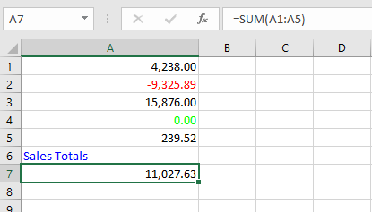
You can use up to four sections within your format string.  Each section is delimited by a semicolon (;). The four sections correspond to positive, negative, zero, and text

Range("A1:A7").NumberFormat = "#,##0.00;[Red]-#,##0.00;[Green] #,##0.00;[Blue]”

In this example, we use the same hash, comma, and zero characters to provide thousand separators and two decimal points, but we now have different sections for each type of value.

The first section is for positive numbers and is no different to what we have already seen previously in terms of format.

The second section for negative numbers introduces a color (Red) which is held within a pair of square brackets. The format is the same as for positive numbers except that a minus (-) sign has been added in front.

The third section for zero numbers uses a color (Green) within square brackets with the numeric string the same as for positive numbers.

The final section is for text values, and all that this needs is a color (Blue) again within square brackets

This is the result of applying this format string:

You can go further with conditions within the format string.  Suppose that you wanted to show every positive number above 10,000 as green, and every other number as red you could use this format string:

Range("A1:A7").NumberFormat = "[>=10000][Green]#,##0.00;[<10000][Red]#,##0.00"

This format string includes conditions for >=10000 set in square brackets so that green will only be used where the number is greater than or equal to 10000

This is the result:

Using Fractions in Formatting Strings

Fractions are not often used in spreadsheets, since they normally equate to decimals which everyone is familiar with.

However, sometimes they do serve a purpose. This example will display dollars and cents:

Range("A1:A7").NumberFormat = "#,##0 "" dollars and "" 00/100 ""  cents """

This is the result that will be produced:

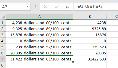
Remember that in spite of the numbers being displayed as text, they are still there in the background as numbers and all the Excel formulas can still be used on them.

Date and Time Formats

Dates are actually numbers and you can use formats on them in the same way as for numbers.  If you format a date as a numeric number, you will see a large number to the left of the decimal point and a number of decimal places. The number to the left of the decimal point shows the number of days starting at 01-Jan-1900, and the decimal places show the time based on 24hrs

MsgBox Format(Now(), "dd-mmm-yyyy")

This will format the current date to show ’08-Jul-2020’. Using ‘mmm’ for the month displays the first three characters of the month name.  If you want the full month name then you use ‘mmmm’

You can include times in your format string:

MsgBox Format(Now(), "dd-mmm-yyyy hh:mm AM/PM")

This will display ’08-Jul-2020 01:25 PM’

‘hh:mm’ represents hours and minutes and AM/PM uses a 12-hour clock as opposed to a 24-hour clock.

You can incorporate text characters into your format string:

MsgBox Format(Now(), "dd-mmm-yyyy hh:mm AM/PM"" today""")

This will display ’08-Jul-2020 01:25 PM today’

You can also use literal characters using a backslash in front in the same way as for numeric format strings.

VBA Programming | Code Generator does work for you!

Predefined Formats

Excel has a number of built-in formats for both numbers and dates that you can use in your code.  These mainly reflect what is available on the number formatting front end, although some of them go beyond what is normally available on the pop-up window.  Also, you do not have the flexibility over number of decimal places, or whether thousands separators are used.

General Number

This format will display the number exactly as it is

MsgBox Format(1234567.89, "General Number")

The result will be 1234567.89

Currency

MsgBox Format(1234567.894, "Currency")

This format will add a currency symbol in front of the number e.g. $, £ depending on your locale, but it will also format the number to 2 decimal places and will separate the thousands with commas.

The result will be $1,234,567.89

Fixed

MsgBox Format(1234567.894, "Fixed")

This format displays at least one digit to the left but only two digits to the right of the decimal point.

The result will be 1234567.89

Standard

MsgBox Format(1234567.894, "Standard")

This displays the number with the thousand separators, but only to two decimal places.

The result will be 1,234,567.89

AutoMacro | Ultimate VBA Add-in | Click for Free Trial!

Percent

MsgBox Format(1234567.894, "Percent")

The number is multiplied by 100 and a percentage symbol (%) is added at the end of the number.  The format displays to 2 decimal places

The result will be 123456789.40%

Scientific

MsgBox Format(1234567.894, "Scientific")

This converts the number to Exponential format

The result will be 1.23E+06

Yes/No

MsgBox Format(1234567.894, "Yes/No")

This displays ‘No’ if the number is zero, otherwise displays ‘Yes’

The result will be ‘Yes’

True/False

MsgBox Format(1234567.894, "True/False")

This displays ‘False’ if the number is zero, otherwise displays ‘True’

The result will be ‘True’

AutoMacro | Ultimate VBA Add-in | Click for Free Trial!

On/Off

MsgBox Format(1234567.894, "On/Off")

This displays ‘Off’ if the number is zero, otherwise displays ‘On’

The result will be ‘On’

General Date

MsgBox Format(Now(), "General Date")

This will display the date as date and time using AM/PM notation.  How the date is displayed depends on your settings in the Windows Control Panel (Clock and Region | Region). It may be displayed as ‘mm/dd/yyyy’ or ‘dd/mm/yyyy’

The result will be ‘7/7/2020 3:48:25 PM’

Long Date

MsgBox Format(Now(), "Long Date")

This will display a long date as defined in the Windows Control Panel (Clock and Region | Region).  Note that it does not include the time.

The result will be ‘Tuesday, July 7, 2020’

Medium Date

MsgBox Format(Now(), "Medium Date")

This displays a date as defined in the short date settings as defined by locale in the Windows Control Panel.

The result will be ’07-Jul-20’

AutoMacro | Ultimate VBA Add-in | Click for Free Trial!

Short Date

MsgBox Format(Now(), "Short Date")

Displays a short date as defined in the Windows Control Panel (Clock and Region | Region). How the date is displayed depends on your locale. It may be displayed as ‘mm/dd/yyyy’ or ‘dd/mm/yyyy’

The result will be ‘7/7/2020’

Long Time

MsgBox Format(Now(), "Long Time")

Displays a long time as defined in Windows Control Panel (Clock and Region | Region).

The result will be ‘4:11:39 PM’

Medium Time

MsgBox Format(Now(), "Medium Time")

Displays a medium time as defined by your locale in the Windows Control Panel. This is usually set as 12-hour format using hours, minutes, and seconds and the AM/PM format.

The result will be ’04:15 PM’

Short Time

MsgBox Format(Now(), "Short Time")

Displays a medium time as defined in Windows Control Panel (Clock and Region | Region). This is usually set as 24-hour format with hours and minutes

The result will be ’16:18’

AutoMacro | Ultimate VBA Add-in | Click for Free Trial!

Dangers of Using Excel’s Pre-Defined Formats in Dates and Times

The use of the pre-defined formats for dates and times in Excel VBA is very dependent on the settings in the Windows Control Panel and also what the locale is set to

Users can easily alter these settings, and this will have an effect on how your dates and times are displayed in Excel

For example, if you develop an Excel application which uses pre-defined formats within your VBA code, these may change completely if a user is in a different country or using a different locale to you.  You may find that column widths do not fit the date definition, or on a user form the Active X control such as a combo box (drop down) control is too narrow for the dates and times to be displayed properly.

You need to consider where the audience is geographically when you develop your Excel application

User-Defined Formats for Numbers

There are a number of different parameters that you can use when defining your format string:

Character	Description
Null String	No formatting
0	Digit placeholder. Displays a digit or a zero. If there is a digit for that position then it displays the digit otherwise it displays 0. If there are fewer digits than zeros, then you will get leading or trailing zeros. If there are more digits after the decimal point than there are zeros, then the number is rounded to the number of decimal places shown by the zeros. If there are more digits before the decimal point than zeros these will be displayed normally.
#	Digit placeholder. This displays a digit or nothing. It works the same as the zero placeholder above, except that leading and trailing zeros are not displayed. For example 0.75 would be displayed using zero placeholders, but this would be .75 using # placeholders.
. Decimal point.	Only one permitted per format string. This character depends on the settings in the Windows Control Panel.
%	Percentage placeholder. Multiplies number by 100 and places % character where it appears in the format string
, (comma)	Thousand separator. This is used if 0 or # placeholders are used and the format string contains a comma. One comma to the left of the decimal point indicates round to the nearest thousand. E.g. ##0, Two adjacent commas to the left of the thousand separator indicate rounding to the nearest million. E.g. ##0,,
E- E+	Scientific format. This displays the number exponentially.
: (colon)	Time separator – used when formatting a time to split hours, minutes and seconds.
/	Date separator – this is used when specifying a format for a date
– + £ $ ( )	Displays a literal character. To display a character other than listed here, precede it with a backslash ()

User-Defined Formats for Dates and Times

These characters can all be used in you format string when formatting dates and times:

Character	Meaning
c	Displays the date as ddddd and the time as ttttt
d	Display the day as a number without leading zero
dd	Display the day as a number with leading zero
ddd	Display the day as an abbreviation (Sun – Sat)
dddd	Display the full name of the day (Sunday – Saturday)
ddddd	Display a date serial number as a complete date according to Short Date in the International settings of the windows Control Panel
dddddd	Displays a date serial number as a complete date according to Long Date in the International settings of the Windows Control Panel.
w	Displays the day of the week as a number (1 = Sunday)
ww	Displays the week of the year as a number (1-53)
m	Displays the month as a number without leading zero
mm	Displays the month as a number with leading zeros
mmm	Displays month as an abbreviation (Jan-Dec)
mmmm	Displays the full name of the month (January – December)
q	Displays the quarter of the year as a number (1-4)
y	Displays the day of the year as a number (1-366)
yy	Displays the year as a two-digit number
yyyy	Displays the year as four-digit number
h	Displays the hour as a number without leading zero
hh	Displays the hour as a number with leading zero
n	Displays the minute as a number without leading zero
nn	Displays the minute as a number with leading zero
s	Displays the second as a number without leading zero
ss	Displays the second as a number with leading zero
ttttt	Display a time serial number as a complete time.
AM/PM	Use a 12-hour clock and display AM or PM to indicate before or after noon.
am/pm	Use a 12-hour clock and use am or pm to indicate before or after noon
A/P	Use a 12-hour clock and use A or P to indicate before or after noon
a/p	Use a 12-hour clock and use a or p to indicate before or after noon

Преобразование чисел, дат и строк в настраиваемый текстовый формат из кода VBA Excel с помощью функции Format. Синтаксис, параметры, символы, примеры.

Format – это функция, которая преобразует число, дату или строку в текст, отформатированный в соответствии с именованным выражением формата или инструкциями, составленными из специальных символов.

Синтаксис и параметры

Format(Expression, [FormatExpression], [FirstDayOfWeek], [FirstWeekOfYear])

• Expression – любое допустимое выражение (переменная), возвращающее числовое значение или строку (обязательный параметр).
• FormatExpression – выражение формата, именованное или содержащее инструкции из специальных символов (необязательный параметр).
• FirstDayOfWeek – константа, задающая первый день недели (необязательный параметр).
• FirstWeekOfYear – константа, задающая первую неделю года (необязательный параметр).

Именованные выражения форматов

Именные форматы даты и времени

Имя формата	Описание
General Date	Стандартное отображение даты и времени в соответствии с параметрами системы.
Long Date	Длинный формат даты.
Medium Date	Средний формат даты.
Short Date	Краткий формат даты.
Long Time	Длинный формат времени.
Medium Time	Средний формат времени.
Short Time	Краткий формат времени.

Проверьте отображение даты и времени с использованием именованных форматов на вашем компьютере при помощи следующего кода VBA Excel:

Sub FormatDateTime() MsgBox «General Date:  « & Format(Now, «General Date») & vbNewLine _ & vbNewLine & «Long Date:  « & Format(Now, «Long Date») & vbNewLine _ & vbNewLine & «Medium Date:  « & Format(Now, «Medium Date») & vbNewLine _ & vbNewLine & «Short Date:  « & Format(Now, «Short Date») & vbNewLine _ & vbNewLine & «Long Time:  « & Format(Now, «Long Time») & vbNewLine _ & vbNewLine & «Medium Time:  « & Format(Now, «Medium Time») & vbNewLine _ & vbNewLine & «Short Time:  « & Format(Now, «Short Time») End Sub

Скорее всего, результат будет таким:

Именованные форматы чисел

Имя формата	Описание
General Number	Стандартное отображение числа без знака разделителя групп разрядов.
Currency	Денежный формат.
Fixed	Отображение числа без знака разделителя групп разрядов с двумя цифрами после разделителя целой и дробной части.
Standard	Отображение числа со знаком разделителя групп разрядов и с двумя цифрами после разделителя целой и дробной части.
Percent	Процентный формат: отображение числа, умноженного на 100, со знаком процента (%), добавленного справа.
Scientific	Отображение числа в экспоненциальном виде.
Yes/No	Возвращается «Нет», если число равно 0, иначе отображается «Да».
True/False	Возвращается «Ложь», если число равно 0, иначе отображается «Истина».
On/Off	Возвращается «Выкл», если число равно 0, иначе отображается «Вкл».

Проверяем работу именованных форматов на числах 2641387.7381962 и 0 с помощью кода VBA Excel:

Sub FormatNumber() Dim n As Double n = 2641387.7381962 ‘n = 0 MsgBox «Форматируемое число = « & n & vbNewLine _ & vbNewLine & «General Number:  « & Format(n, «General Number») & vbNewLine _ & vbNewLine & «Currency:  « & Format(n, «Currency») & vbNewLine _ & vbNewLine & «Fixed:  « & Format(n, «Fixed») & vbNewLine _ & vbNewLine & «Standard:  « & Format(n, «Standard») & vbNewLine _ & vbNewLine & «Percent:  « & Format(n, «Percent») & vbNewLine _ & vbNewLine & «Scientific:  « & Format(n, «Scientific») & vbNewLine _ & vbNewLine & «Yes/No:  « & Format(n, «Yes/No») & vbNewLine _ & vbNewLine & «True/False:  « & Format(n, «True/False») & vbNewLine _ & vbNewLine & «On/Off:  « & Format(n, «On/Off») End Sub

Получаем следующий результат:

 

Вместо вопросительного знака в отображении числа в формате Currency, по идее, должен быть знак валюты (₽ или руб.).

Специальные символы для выражений форматов

Символы для форматов даты и времени

Символ	Описание
Точка (.)	Разделитель компонентов даты (день, месяц, год). Используется при отображении месяца в виде числа.
Пробел	Разделитель компонентов даты (день, месяц, год). Используется при отображении месяца прописью.
Двоеточие (:)	Разделитель компонентов времени (часы, минуты, секунды).
d	День в виде числа без нуля в начале (1–31).
dd	День в виде числа с нулем в начале (01–31).
m	Месяц в виде числа без нуля в начале (1–12). Если (m) следует после (h) или (hh), отображаются минуты (0–59).
mm	Месяц в виде числа с нулем в начале (01–12). Если (mm) следует после (h) или (hh), отображаются минуты (00–59).
mmm	Месяц прописью в сокращенном виде (янв–дек).
mmmm	Полное название месяца (январь–декабрь).
y	День года в виде числа (1–366).
yy	Год в виде 2-значного числа (00–99).
yyyy	Год в виде 4-значного числа (1900–9999).
h	Часы в виде числа без нуля в начале (0–23).
hh	Часы в виде числа с нулем в начале (00–23).
n (m)	Минуты в виде числа без нуля в начале (0–59).
nn (mm)	Минуты в виде числа с нулем в начале (00–59).
s	Секунды в виде числа без нуля в начале (0–59).
ss	Секунды в виде числа с нулем в начале (00–59).

В этой таблице перечислены далеко не все символы для выражений форматов даты и времени. Вы можете ознакомиться со всеми символами, в том числе и для форматирования чисел, на сайте разработчика.

Примеры отображения даты с помощью разных по количеству наборов символа d:

Sub DataIsD() MsgBox «d:  « & Format(Now, «d») & vbNewLine _ & vbNewLine & «dd:  « & Format(Now, «dd») & vbNewLine _ & vbNewLine & «ddd:  « & Format(Now, «ddd») & vbNewLine _ & vbNewLine & «dddd:  « & Format(Now, «dddd») & vbNewLine _ & vbNewLine & «ddddd:  « & Format(Now, «ddddd») & vbNewLine _ & vbNewLine & «dddddd:  « & Format(Now, «dddddd») End Sub

Символы для числовых форматов

Символ	Описание
Точка (.)	Десятичный разделитель.
Запятая (,)	Разделитель групп разрядов. В отображаемых числах заполняется пробелом.
(0)	Заполнитель, который отображает цифру или ноль. Используется, когда нужны ведущие нули или нули в конце числа.
(#)	Заполнитель, который отображает цифру или ничего не отображает. Используется, когда не нужны ведущие нули или нули в конце числа.
(%)	Заполнитель процента. Выражение умножается на 100, а знак процента (%) вставляется на той позиции, где он указан в строке формата.
(E- E+ e- e+)	Экспоненциальный формат.

Примеры использования символов в выражениях числовых форматов VBA Excel:

Sub FormatNumber2() Dim n As Double n = 2641387.7381962 ‘n = 0.2397842 MsgBox «Форматируемое число = « & n & vbNewLine _ & vbNewLine & «0.##:  « & Format(n, «0.##») & vbNewLine _ & vbNewLine & «000.###:  « & Format(n, «000.###») & vbNewLine _ & vbNewLine & «#,###.###:  « & Format(n, «#,###.###») & vbNewLine _ & vbNewLine & «0 %:  « & Format(n, «0 %») & vbNewLine _ & vbNewLine & «0.### E-:  « & Format(n, «0.### E-«) & vbNewLine _ & vbNewLine & «0.### E+:  « & Format(n, «0.### E+») End Sub

 

Символы для текстовых форматов

Символ	Описание
At-символ (@)	Заполнитель для символов, отображающий знак или пробел.
Амперсанд (&)	Заполнитель для символов, отображающий знак или ничего (пустая строка).
Меньше (<)	Принудительный перевод всех буквенных символов в нижний регистр.
Больше (>)	Принудительный перевод всех буквенных символов в верхний регистр.

Примеры использования символов в выражениях строковых форматов VBA Excel:

Sub FormatString() MsgBox «Номер телефона:  « & Format(«1234567890», «+7 (@@@) @@@-@@-@@») & vbNewLine _ & vbNewLine & «Серия и номер паспорта:  « & Format(«1234567890», «&& && &&&&») & vbNewLine _ & vbNewLine & «Нижний регистр:  « & Format(«Нижний регистр», «<«) & vbNewLine _ & vbNewLine & «Верхний регистр: « & Format(«Верхний регистр», «>») End Sub

Форматы для различных значений одного выражения

Различные форматы для разных числовых значений

В выражении формата для чисел предусмотрено от одного до четырех разделов, отделяемых друг от друга точкой с запятой. Отображаемая строка зависит от значения, возвращенного параметром Expression функции Format.

Количество разделов	Результат форматирования
Один раздел	Выражение формата применяется ко всем значениям.
Два раздела	Первый раздел применяется к положительным значениям и нулям, второй – к отрицательным значениям.
Три раздела	Первый раздел применяется к положительным значениям, второй – к отрицательным значениям, третий – к нулям.
Четыре раздела	Первый раздел применяется к положительным значениям, второй – к отрицательным значениям, третий – к нулям, четвертый – к значениям Null.

Пример использования четырех разделов в выражении формата числовых значений:

Sub FormatDifferentValues() MsgBox «Число 1234,5678:  « & _ Format(1234.5678, «#,##0.00 руб.;Отрицательное число;Ноль рублей;Значение Null») _ & vbNewLine & vbNewLine & «Число -25:  « & _ Format(—25, «#,##0.00 руб.;Отрицательное число;Ноль рублей;Значение Null») _ & vbNewLine & vbNewLine & «Число 0:  « & _ Format(0, «#,##0.00 руб.;Отрицательное число;Ноль рублей;Значение Null») _ & vbNewLine & vbNewLine & «Null:  « & _ Format(Null, «#,##0.00 руб.;Отрицательное число;Ноль рублей;Значение Null») End Sub

Различные форматы для разных строковых значений

В выражении формата для строк предусмотрено до двух разделов, отделяемых друг от друга точкой с запятой. Отображаемая строка зависит от текста, возвращенного параметром Expression функции Format.

Количество разделов	Результат форматирования
Один раздел	Выражение формата применяется ко всем строковым данным.
Два раздела	Первый раздел применяется к строковым данным, второй – к значениям Null и пустым строкам («»).

Пример использования двух разделов в выражении формата строк:

Sub FormatString2() MsgBox «Строка «Белка»:  « & _ Format(«Белка», «@;Пустая строка или Null») _ & vbNewLine & vbNewLine & «Пустая строка:  « & _ Format(«», «@;Пустая строка или Null») _ & vbNewLine & vbNewLine & «Строка «Null»:  « & _ Format(«Null», «@;Пустая строка или Null») _ & vbNewLine & vbNewLine & «Значение Null:  « & _ Format(Null, «@;Пустая строка или Null») End Sub

Formatting Cells Number

General

Range("A1").NumberFormat = "General"

Number

Range("A1").NumberFormat = "0.00"

Currency

Range("A1").NumberFormat = "$#,##0.00"

Accounting

Range("A1").NumberFormat = "_($* #,##0.00_);_($* (#,##0.00);_($* ""-""??_);_(@_)"

Date

Range("A1").NumberFormat = "yyyy-mm-dd;@"

Time

Range("A1").NumberFormat = "h:mm:ss AM/PM;@"

Percentage

Range("A1").NumberFormat = "0.00%"

Fraction

Range("A1").NumberFormat = "# ?/?"

Scientific

Range("A1").NumberFormat = "0.00E+00"

Text

Range("A1").NumberFormat = "@"

Special

Range("A1").NumberFormat = "00000"

Custom

Range("A1").NumberFormat = "$#,##0.00_);[Red]($#,##0.00)"

Formatting Cells Alignment

Text Alignment

Horizontal

The value of this property can be set to one of the constants: xlGeneral, xlCenter, xlDistributed, xlJustify, xlLeft, xlRight.

The following code sets the horizontal alignment of cell A1 to center.

Range("A1").HorizontalAlignment = xlCenter

Vertical

The value of this property can be set to one of the constants: xlBottom, xlCenter, xlDistributed, xlJustify, xlTop.

The following code sets the vertical alignment of cell A1 to bottom.

Range("A1").VerticalAlignment = xlBottom

Text Control

Wrap Text

This example formats cell A1 so that the text wraps within the cell.

Range("A1").WrapText = True

Shrink To Fit

This example causes text in row one to automatically shrink to fit in the available column width.

Rows(1).ShrinkToFit = True

Merge Cells

This example merge range A1:A4 to a large one.

Range("A1:A4").MergeCells = True

Right-to-left

Text direction

The value of this property can be set to one of the constants: xlRTL (right-to-left), xlLTR (left-to-right), or xlContext (context).

The following code example sets the reading order of cell A1 to xlRTL (right-to-left).

Range("A1").ReadingOrder = xlRTL

Orientation

The value of this property can be set to an integer value from –90 to 90 degrees or to one of the following constants: xlDownward, xlHorizontal, xlUpward, xlVertical.

The following code example sets the orientation of cell A1 to xlHorizontal.

Range("A1").Orientation = xlHorizontal

Font

Font Name

The value of this property can be set to one of the fonts: Calibri, Times new Roman, Arial…

The following code sets the font name of range A1:A5 to Calibri.

Range("A1:A5").Font.Name = "Calibri"

Font Style

The value of this property can be set to one of the constants: Regular, Bold, Italic, Bold Italic.

The following code sets the font style of range A1:A5 to Italic.

Range("A1:A5").Font.FontStyle = "Italic"

Font Size

The value of this property can be set to an integer value from 1 to 409.

The following code sets the font size of cell A1 to 14.

Range("A1").Font.Size = 14

Underline

The value of this property can be set to one of the constants: xlUnderlineStyleNone, xlUnderlineStyleSingle, xlUnderlineStyleDouble, xlUnderlineStyleSingleAccounting, xlUnderlineStyleDoubleAccounting.

The following code sets the font of cell A1 to xlUnderlineStyleDouble (double underline).

Range("A1").Font.Underline = xlUnderlineStyleDouble

Font Color

The value of this property can be set to one of the standard colors: vbBlack, vbRed, vbGreen, vbYellow, vbBlue, vbMagenta, vbCyan, vbWhite or an integer value from 0 to 16,581,375.

To assist you with specifying the color of anything, the VBA is equipped with a function named RGB. Its syntax is:

Function RGB(RedValue As Byte, GreenValue As Byte, BlueValue As Byte) As long

This function takes three arguments and each must hold a value between 0 and 255. The first argument represents the ratio of red of the color. The second argument represents the green ratio of the color. The last argument represents the blue of the color. After the function has been called, it produces a number whose maximum value can be 255 * 255 * 255 = 16,581,375, which represents a color.

The following code sets the font color of cell A1 to vbBlack (Black).

Range("A1").Font.Color = vbBlack

The following code sets the font color of cell A1 to 0 (Black).

Range("A1").Font.Color = 0

The following code sets the font color of cell A1 to RGB(0, 0, 0) (Black).

Range("A1").Font.Color = RGB(0, 0, 0)

Font Effects

Strikethrough

True if the font is struck through with a horizontal line.

The following code sets the font of cell A1 to strikethrough.

Range("A1").Font.Strikethrough = True

Subscript

True if the font is formatted as subscript. False by default.

The following code sets the font of cell A1 to Subscript.

Range("A1").Font.Subscript = True

Superscript

True if the font is formatted as superscript; False by default.

The following code sets the font of cell A1 to Superscript.

Range("A1").Font.Superscript = True

Border

Border Index

Using VBA you can choose to create borders for the different edges of a range of cells:

1. xlDiagonalDown (Border running from the upper left-hand corner to the lower right of each cell in the range).
2. xlDiagonalUp (Border running from the lower left-hand corner to the upper right of each cell in the range).
3. xlEdgeBottom (Border at the bottom of the range).
4. xlEdgeLeft (Border at the left-hand edge of the range).
5. xlEdgeRight (Border at the right-hand edge of the range).
6. xlEdgeTop (Border at the top of the range).
7. xlInsideHorizontal (Horizontal borders for all cells in the range except borders on the outside of the range).
8. xlInsideVertical (Vertical borders for all the cells in the range except borders on the outside of the range).

Line Style

The value of this property can be set to one of the constants: xlContinuous (Continuous line), xlDash (Dashed line), xlDashDot (Alternating dashes and dots), xlDashDotDot (Dash followed by two dots), xlDot (Dotted line), xlDouble (Double line), xlLineStyleNone (No line), xlSlantDashDot (Slanted dashes).

The following code example sets the border on the bottom edge of cell A1 with continuous line.

Range("A1").Borders(xlEdgeBottom).LineStyle = xlContinuous

The following code example removes the border on the bottom edge of cell A1.

Range("A1").Borders(xlEdgeBottom).LineStyle = xlNone

Line Thickness

The value of this property can be set to one of the constants: xlHairline (Hairline, thinnest border), xlMedium (Medium), xlThick (Thick, widest border), xlThin (Thin).

The following code example sets the thickness of the border created to xlThin (Thin).

Range("A1").Borders(xlEdgeBottom).Weight = xlThin

Line Color

The value of this property can be set to one of the standard colors: vbBlack, vbRed, vbGreen, vbYellow, vbBlue, vbMagenta, vbCyan, vbWhite or an integer value from 0 to 16,581,375.

The following code example sets the color of the border on the bottom edge to green.

Range("A1").Borders(xlEdgeBottom).Color = vbGreen

You can also use the RGB function to create a color value.

The following example sets the color of the bottom border of cell A1 with RGB fuction.

Range("A1").Borders(xlEdgeBottom).Color = RGB(255, 0, 0)

Fill

Pattern Style

The value of this property can be set to one of the constants:

1. xlPatternAutomatic (Excel controls the pattern.)
2. xlPatternChecker (Checkerboard.)
3. xlPatternCrissCross (Criss-cross lines.)
4. xlPatternDown (Dark diagonal lines running from the upper left to the lower right.)
5. xlPatternGray16 (16% gray.)
6. xlPatternGray25 (25% gray.)
7. xlPatternGray50 (50% gray.)
8. xlPatternGray75 (75% gray.)
9. xlPatternGray8 (8% gray.)
10. xlPatternGrid (Grid.)
11. xlPatternHorizontal (Dark horizontal lines.)
12. xlPatternLightDown (Light diagonal lines running from the upper left to the lower right.)
13. xlPatternLightHorizontal (Light horizontal lines.)
14. xlPatternLightUp (Light diagonal lines running from the lower left to the upper right.)
15. xlPatternLightVertical (Light vertical bars.)
16. xlPatternNone (No pattern.)
17. xlPatternSemiGray75 (75% dark moiré.)
18. xlPatternSolid (Solid color.)
19. xlPatternUp (Dark diagonal lines running from the lower left to the upper right.)

Protection

Locking Cells

This property returns True if the object is locked, False if the object can be modified when the sheet is protected, or Null if the specified range contains both locked and unlocked cells.

The following code example unlocks cells A1:B22 on Sheet1 so that they can be modified when the sheet is protected.

Worksheets("Sheet1").Range("A1:B22").Locked = False
Worksheets("Sheet1").Protect

Hiding Formulas

This property returns True if the formula will be hidden when the worksheet is protected, Null if the specified range contains some cells with FormulaHidden equal to True and some cells with FormulaHidden equal to False.

Don’t confuse this property with the Hidden property. The formula will not be hidden if the workbook is protected and the worksheet is not, but only if the worksheet is protected.

The following code example hides the formulas in cells A1 and C1 on Sheet1 when the worksheet is protected.

Worksheets("Sheet1").Range("A1:C1").FormulaHidden = True

VBA Format Cells

In this Article

This tutorial will demonstrate how to format cells using VBA.

Formatting Cells

There are many formatting properties that can be set for a (range of) cells like this:

Let’s see them in alphabetical order:

AddIndent

By setting the value of this property to True the text will be automatically indented when the text alignment in the cell is set, either horizontally or vertically, to equal distribution (see HorizontalAlignment and VerticalAlignment).

Borders

You can set the border format of a cell. See here for more information about borders.

As an example you can set a red dashed line around cell B2 on Sheet 1 like this:

You can adjust the cell’s font format by setting the font name, style, size, color, adding underlines and or effects (strikethrough, sub- or superscript). See here for more information about cell fonts.

Here are some examples:

FormulaHidden

This property returns or sets a variant value that indicates if the formula will be hidden when the worksheet is protected. For example:

HorizontalAlignment

This property cell format property returns or sets a variant value that represents the horizontal alignment for the specified object. Returned or set constants can be: xlGeneral, xlCenter, xlDistributed, xlJustify, xlLeft, xlRight, xlFill, xlCenterAcrossSelection. For example:

VBA Coding Made Easy

Stop searching for VBA code online. Learn more about AutoMacro — A VBA Code Builder that allows beginners to code procedures from scratch with minimal coding knowledge and with many time-saving features for all users!

IndentLevel

It returns or sets an integer value between 0 and 15 that represents the indent level for the cell or range.

Interior

You can set or get returned information about the cell’s interior: its Color, ColorIndex, Pattern, PatternColor, PatternColorIndex, PatternThemeColor, PatternTintAndShade, ThemeColor, TintAndShade, like this:

Locked

This property returns True if the cell or range is locked, False if the object can be modified when the sheet is protected, or Null if the specified range contains both locked and unlocked cells. It can be used also for locking or unlocking cells.

This example unlocks cells A1:B2 on Sheet1 so that they can be modified when the sheet is protected.

MergeCells

Set this property to True if you need to merge a range. Its value gets True if a specified range contains merged cells. For example, if you need to merge the range of C5:D7, you can use this code:

NumberFormat

You can set the number format within the cell(s) to General, Number, Currency, Accounting, Date, Time, Percentage, Fraction, Scientific, Text, Special and Custom.

Here are the examples of scientific and percentage number formats:

NumberFormatLocal

This property returns or sets a variant value that represents the format code for the object as a string in the language of the user.

Orientation

You can set (or get returned) the text orientation within the cell(s) by this property. Its value can be one of these constants: xlDownward, xlHorizontal, xlUpward, xlVertical or an integer value from –90 to 90 degrees.

Parent

This is a read-only property that returns the parent object of a specified object.

ShrinkToFit

This property returns or sets a variant value that indicates if text automatically shrinks to fit in the available column width.

VerticalAlignment

This property cell format property returns or sets a variant value that represents the vertical alignment for the specified object. Returned or set constants can be: xlCenter, xlDistributed, xlJustify, xlBottom, xlTop. For example:

WrapText

This property returns True if text is wrapped in all cells within the specified range, False if text is not wrapped in all cells within the specified range, or Null if the specified range contains some cells that wrap text and other cells that don’t.

For example, if you have this range of cells: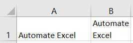

this code below will return Null in the Immediate Window:

VBA Code Examples Add-in

Easily access all of the code examples found on our site.

Simply navigate to the menu, click, and the code will be inserted directly into your module. .xlam add-in.

Источник

VBA Excel. Свойства ячейки (объекта Range)

Свойства ячейки, часто используемые в коде VBA Excel. Демонстрация свойств ячейки, как структурной единицы объекта Range, на простых примерах.

Ячейка и объект Range

Объект Range в VBA Excel представляет диапазон ячеек. Он (объект Range) может описывать любой диапазон, начиная от одной ячейки и заканчивая сразу всеми ячейками рабочего листа.

• Одна ячейка – Range(«A1») .
• Девять ячеек – Range(«A1:С3») .
• Весь рабочий лист в Excel 2016 – Range(«1:1048576») .

В VBA Excel есть свойство Cells объекта Range, которое позволяет обратиться к одной ячейке в указанном диапазоне (возвращает объект Range в виде одной ячейки). Если в коде используется свойство Cells без указания диапазона, значит оно относится ко всему диапазону активного рабочего листа.

Примеры обращения к одной ячейке:

• Cells(1000) , где 1000 – порядковый номер ячейки на рабочем листе, возвращает ячейку «ALL1».
• Cells(50, 20) , где 50 – номер строки рабочего листа, а 20 – номер столбца, возвращает ячейку «T50».
• Range(«A1:C3»).Cells(6) , где «A1:C3» – заданный диапазон, а 6 – порядковый номер ячейки в этом диапазоне, возвращает ячейку «C2».

Подробнее о том, как обратиться к ячейке, смотрите в статье: Ячейки (обращение, запись, чтение, очистка).

В этой статье мы рассмотрим свойства объекта Range, применимые, в том числе, к диапазону, состоящему из одной ячейки.

Еще надо добавить, что свойства и методы объектов отделяются от объектов точкой, как в третьем примере обращения к одной ячейке: Range(«A1:C3»).Cells(6) .

Свойства ячейки (объекта Range)

Свойство	Описание
Address	Возвращает адрес ячейки (диапазона).
Borders	Возвращает коллекцию Borders, представляющую границы ячейки (диапазона). Подробнее…
Cells	Возвращает объект Range, представляющий коллекцию всех ячеек заданного диапазона. Указав номер строки и номер столбца или порядковый номер ячейки в диапазоне, мы получаем конкретную ячейку. Подробнее…
Characters	Возвращает подстроку в размере указанного количества символов из текста, содержащегося в ячейке. Подробнее…
Column	Возвращает номер столбца ячейки (первого столбца диапазона). Подробнее…
ColumnWidth	Возвращает или задает ширину ячейки в пунктах (ширину всех столбцов в указанном диапазоне).
Comment	Возвращает комментарий, связанный с ячейкой (с левой верхней ячейкой диапазона).
CurrentRegion	Возвращает прямоугольный диапазон, ограниченный пустыми строками и столбцами. Очень полезное свойство для возвращения рабочей таблицы, а также определения номера последней заполненной строки.
EntireColumn	Возвращает весь столбец (столбцы), в котором содержится ячейка (диапазон). Диапазон может содержаться и в одном столбце, например, Range(«A1:A20») .
EntireRow	Возвращает всю строку (строки), в которой содержится ячейка (диапазон). Диапазон может содержаться и в одной строке, например, Range(«A2:H2») .
Font	Возвращает объект Font, представляющий шрифт указанного объекта. Подробнее о цвете шрифта…
HorizontalAlignment	Возвращает или задает значение горизонтального выравнивания содержимого ячейки (диапазона). Подробнее…
Interior	Возвращает объект Interior, представляющий внутреннюю область ячейки (диапазона). Применяется, главным образом, для возвращения или назначения цвета заливки (фона) ячейки (диапазона). Подробнее…
Name	Возвращает или задает имя ячейки (диапазона).
NumberFormat	Возвращает или задает код числового формата для ячейки (диапазона). Примеры кодов числовых форматов можно посмотреть, открыв для любой ячейки на рабочем листе Excel диалоговое окно «Формат ячеек», на вкладке «(все форматы)». Свойство NumberFormat диапазона возвращает значение NULL, за исключением тех случаев, когда все ячейки в диапазоне имеют одинаковый числовой формат. Если нужно присвоить ячейке текстовый формат, записывается так: Range(«A1»).NumberFormat = «@» . Общий формат: Range(«A1»).NumberFormat = «General» .
Offset	Возвращает объект Range, смещенный относительно первоначального диапазона на указанное количество строк и столбцов. Подробнее…
Resize	Изменяет размер первоначального диапазона до указанного количества строк и столбцов. Строки добавляются или удаляются снизу, столбцы – справа. Подробнее…
Row	Возвращает номер строки ячейки (первой строки диапазона). Подробнее…
RowHeight	Возвращает или задает высоту ячейки в пунктах (высоту всех строк в указанном диапазоне).
Text	Возвращает форматированный текст, содержащийся в ячейке. Свойство Text диапазона возвращает значение NULL, за исключением тех случаев, когда все ячейки в диапазоне имеют одинаковое содержимое и один формат. Предназначено только для чтения. Подробнее…
Value	Возвращает или задает значение ячейки, в том числе с отображением значений в формате Currency и Date. Тип данных Variant. Value является свойством ячейки по умолчанию, поэтому в коде его можно не указывать.
Value2	Возвращает или задает значение ячейки. Тип данных Variant. Значения в формате Currency и Date будут отображены в виде чисел с типом данных Double.
VerticalAlignment	Возвращает или задает значение вертикального выравнивания содержимого ячейки (диапазона). Подробнее…

В таблице представлены не все свойства объекта Range. С полным списком вы можете ознакомиться не сайте разработчика.

Простые примеры для начинающих

Вы можете скопировать примеры кода VBA Excel в стандартный модуль и запустить их на выполнение. Как создать стандартный модуль и запустить процедуру на выполнение, смотрите в статье VBA Excel. Начинаем программировать с нуля.

Учтите, что в одном программном модуле у всех процедур должны быть разные имена. Если вы уже копировали в модуль подпрограммы с именами Primer1, Primer2 и т.д., удалите их или создайте еще один стандартный модуль.

Форматирование ячеек

Заливка ячейки фоном, изменение высоты строки, запись в ячейки текста, автоподбор ширины столбца, выравнивание текста в ячейке и выделение его цветом, добавление границ к ячейкам, очистка содержимого и форматирования ячеек.

Если вы запустите эту процедуру, информационное окно MsgBox будет прерывать выполнение программы и сообщать о том, что произойдет дальше, после его закрытия.

Источник

VBA-Урок 5. Свойства (Properties)

В данной статье мы будем учиться писать VBA код, чтобы управлять содержимым ячеек, самими ячейками и листами.

1. Запись значений в ячейку

Для начала откроем редактор, добавим модуль, скопируем туда этот макрос:

Мы обратились к ячейке A1 . Теперь давайте попробуем управлять данной ячейкой. Чтобы увидеть, что мы можем сделать, добавим точку после Range («A1»).

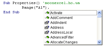
Выберите значение Value и нажмите Tab. Получим такой код:

Значение Value отображает содержимое ячейки.

Теперь давайте запишем значение 35 в ячейку A1:

Попробуем теперь записать текст в ячейку (когда присваиваем текстовое значение, его нужно брать в двойные кавычки «»):

Заметим, что макрос будет отображать значение в том листе, который вы последний раз открывали. Поэтому, чтобы управлять содержимым ячейки на любом листе книги, нам нужно будет прописать полный путь к ячейке, а именно добавить впереди кода название листа, например:

Вариант 1. Обращаемся по названию листа — Sheets(«Sheet2»).

Вариант 2. Обращаемся не по названию листа, а по его порядковому номеру — Sheets(2).

Аналогично, если мы хотим обратиться к ячейке в другой книге, нам нужно в начале кода прописать название книги:

Хотя мы указываем параметр Value в наших примерах, на самом деле его можно не использовать, поскольку он стоит по умолчанию. То есть, эти две строки кода будут эквивалентными:

2. Удаление значений

Удалим значение 35 из ячейки A1, которое мы записали в начале урока:

3. Форматирование значений

Если вы выберете значение Font , то появится список параметров, которые вы сможете применить к ячейке:

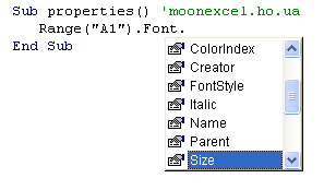
Форматирование: изменение размера текста

Давайте присвоим ячейке значение 35 и уменьшим размер шрифта до 8:

Источник

Formatting Numbers in Excel VBA

In this Article

Formatting Numbers in Excel VBA

Numbers come in all kinds of formats in Excel worksheets. You may already be familiar with the pop-up window in Excel for making use of different numerical formats:

Formatting of numbers make the numbers easier to read and understand. The Excel default for numbers entered into cells is ‘General’ format, which means that the number is displayed exactly as you typed it in.

For example, if you enter a round number e.g. 4238, it will be displayed as 4238 with no decimal point or thousands separators. A decimal number such as 9325.89 will be displayed with the decimal point and the decimals. This means that it will not line up in the column with the round numbers, and will look extremely messy.

Also, without showing the thousands separators, it is difficult to see how large a number actually is without counting the individual digits. Is it in millions or tens of millions?

From the point of view of a user looking down a column of numbers, this makes it quite difficult to read and compare.

In VBA you have access to exactly the same range of formats that you have on the front end of Excel. This applies to not only an entered value in a cell on a worksheet, but also things like message boxes, UserForm controls, charts and graphs, and the Excel status bar at the bottom left hand corner of the worksheet.

The Format function is an extremely useful function in VBA in presentation terms, but it is also very complex in terms of the flexibility offered in how numbers are displayed.

How to Use the Format Function in VBA

If you are showing a message box, then the Format function can be used directly:

This will display a large number using commas to separate the thousands and to show 2 decimal places. The result will be 1,234,567.89. The zeros in place of the hash ensure that decimals will be shown as 00 in whole numbers, and that there is a leading zero for a number which is less than 1

The hashtag symbol (#) represents a digit placeholder which displays a digit if it is available in that position, or else nothing.

You can also use the format function to address an individual cell, or a range of cells to change the format:

This code will set the range of cells (A1 to A10) to a custom format which separates the thousands with commas and shows 2 decimal places.

If you check the format of the cells on the Excel front end, you will find that a new custom format has been created.

You can also format numbers on the Excel Status Bar at the bottom left hand corner of the Excel window:

You clear this from the status bar by using:

Creating a Format String

This example will add the text ‘Total Sales’ after each number, as well as including a thousands separator

This is what your numbers will look like:

Note that cell A6 has a ‘SUM’ formula, and this will include the ‘Total Sales’ text without requiring formatting. If the formatting is applied, as in the above code, it will not put an extra instance of ‘Total Sales’ into cell A6

Although the cells now display alpha numeric characters, the numbers are still present in numeric form. The ‘SUM’ formula still works because it is using the numeric value in the background, not how the number is formatted.

The comma in the format string provides the thousands separator. Note that you only need to put this in the string once. If the number runs into millions or billions, it will still separate the digits into groups of 3

The zero in the format string (0) is a digit placeholder. It displays a digit if it is there, or a zero. Its positioning is very important to ensure uniformity with the formatting

In the format string, the hash characters (#) will display nothing if there is no digit. However, if there is a number like .8 (all decimals), we want it to show as 0.80 so that it lines up with the other numbers.

By using a single zero to the left of the decimal point and two zeros to the right of the decimal point in the format string, this will give the required result (0.80).

If there was only one zero to the right of the decimal point, then the result would be ‘0.8’ and everything would be displayed to one decimal place.

Using a Format String for Alignment

We may want to see all the decimal numbers in a range aligned on their decimal points, so that all the decimal points are directly under each other, however many places of decimals there are on each number.

You can use a question mark (?) within your format string to do this. The ‘?’ indicates that a number is shown if it is available, or a space

This will display your numbers as follows:

All the decimal points now line up underneath each other. Cell A5 has three decimal places and this would throw the alignment out normally, but using the ‘?’ character aligns everything perfectly.

Using Literal Characters Within the Format String

You can add any literal character into your format string by preceding it with a backslash ().

Suppose that you want to show a particular currency indicator for your numbers which is not based on your locale. The problem is that if you use a currency indicator, Excel automatically refers to your local and changes it to the one appropriate for the locale that is set on the Windows Control Panel. This could have implications if your Excel application is being distributed in other countries and you want to ensure that whatever the locale is, the currency indicator is always the same.

You may also want to indicate that the numbers are in millions in the following example:

This will produce the following results on your worksheet:

In using a backslash to display literal characters, you do not need to use a backslash for each individual character within a string. You can use:

This will display ‘mill’ after every number within the formatted range.

You can use most characters as literals, but not reserved characters such as 0, #,?

Use of Commas in a Format String

We have already seen that commas can be used to create thousands separators for large numbers, but they can also be used in another way.

By using them at the end of the numeric part of the format string, they act as scalers of thousands. In other words, they will divide each number by 1,000 every time there is a comma.

In the example data, we are showing it with an indicator that it is in millions. By inserting one comma into the format string, we can show those numbers divided by 1,000.

This will show the numbers divided by 1,000 although the original number will still be in background in the cell.

If you put two commas in the format string, then the numbers will be divided by a million

This will be the result using only one comma (divide by 1,000):

VBA Coding Made Easy

Stop searching for VBA code online. Learn more about AutoMacro — A VBA Code Builder that allows beginners to code procedures from scratch with minimal coding knowledge and with many time-saving features for all users!

Creating Conditional Formatting within the Format String

You could set up conditional formatting on the front end of Excel, but you can also do it within your VBA code, which means that you can manipulate the format string programmatically to make changes.

You can use up to four sections within your format string. Each section is delimited by a semicolon (;). The four sections correspond to positive, negative, zero, and text

In this example, we use the same hash, comma, and zero characters to provide thousand separators and two decimal points, but we now have different sections for each type of value.

The first section is for positive numbers and is no different to what we have already seen previously in terms of format.

The second section for negative numbers introduces a color (Red) which is held within a pair of square brackets. The format is the same as for positive numbers except that a minus (-) sign has been added in front.

The third section for zero numbers uses a color (Green) within square brackets with the numeric string the same as for positive numbers.

The final section is for text values, and all that this needs is a color (Blue) again within square brackets

This is the result of applying this format string:

You can go further with conditions within the format string. Suppose that you wanted to show every positive number above 10,000 as green, and every other number as red you could use this format string:

This format string includes conditions for >=10000 set in square brackets so that green will only be used where the number is greater than or equal to 10000

This is the result:

Using Fractions in Formatting Strings

Fractions are not often used in spreadsheets, since they normally equate to decimals which everyone is familiar with.

However, sometimes they do serve a purpose. This example will display dollars and cents:

This is the result that will be produced:

Remember that in spite of the numbers being displayed as text, they are still there in the background as numbers and all the Excel formulas can still be used on them.

Date and Time Formats

Dates are actually numbers and you can use formats on them in the same way as for numbers. If you format a date as a numeric number, you will see a large number to the left of the decimal point and a number of decimal places. The number to the left of the decimal point shows the number of days starting at 01-Jan-1900, and the decimal places show the time based on 24hrs

This will format the current date to show ’08-Jul-2020’. Using ‘mmm’ for the month displays the first three characters of the month name. If you want the full month name then you use ‘mmmm’

You can include times in your format string:

This will display ’08-Jul-2020 01:25 PM’

‘hh:mm’ represents hours and minutes and AM/PM uses a 12-hour clock as opposed to a 24-hour clock.

You can incorporate text characters into your format string:

This will display ’08-Jul-2020 01:25 PM today’

You can also use literal characters using a backslash in front in the same way as for numeric format strings.

Predefined Formats

Excel has a number of built-in formats for both numbers and dates that you can use in your code. These mainly reflect what is available on the number formatting front end, although some of them go beyond what is normally available on the pop-up window. Also, you do not have the flexibility over number of decimal places, or whether thousands separators are used.

General Number

This format will display the number exactly as it is

The result will be 1234567.89

Currency

This format will add a currency symbol in front of the number e.g. $, £ depending on your locale, but it will also format the number to 2 decimal places and will separate the thousands with commas.

The result will be $1,234,567.89

Fixed

This format displays at least one digit to the left but only two digits to the right of the decimal point.

The result will be 1234567.89

Standard

This displays the number with the thousand separators, but only to two decimal places.

The result will be 1,234,567.89

Percent

The number is multiplied by 100 and a percentage symbol (%) is added at the end of the number. The format displays to 2 decimal places

The result will be 123456789.40%

Scientific

This converts the number to Exponential format

The result will be 1.23E+06

Yes/No

This displays ‘No’ if the number is zero, otherwise displays ‘Yes’

The result will be ‘Yes’

True/False

This displays ‘False’ if the number is zero, otherwise displays ‘True’

The result will be ‘True’

On/Off

This displays ‘Off’ if the number is zero, otherwise displays ‘On’

The result will be ‘On’

General Date

This will display the date as date and time using AM/PM notation. How the date is displayed depends on your settings in the Windows Control Panel (Clock and Region | Region). It may be displayed as ‘mm/dd/yyyy’ or ‘dd/mm/yyyy’

The result will be ‘7/7/2020 3:48:25 PM’

Long Date

This will display a long date as defined in the Windows Control Panel (Clock and Region | Region). Note that it does not include the time.

The result will be ‘Tuesday, July 7, 2020’

Medium Date

This displays a date as defined in the short date settings as defined by locale in the Windows Control Panel.

The result will be ’07-Jul-20’

Short Date

Displays a short date as defined in the Windows Control Panel (Clock and Region | Region). How the date is displayed depends on your locale. It may be displayed as ‘mm/dd/yyyy’ or ‘dd/mm/yyyy’

The result will be ‘7/7/2020’

Long Time

Displays a long time as defined in Windows Control Panel (Clock and Region | Region).

The result will be ‘4:11:39 PM’

Medium Time

Displays a medium time as defined by your locale in the Windows Control Panel. This is usually set as 12-hour format using hours, minutes, and seconds and the AM/PM format.

The result will be ’04:15 PM’

Short Time

Displays a medium time as defined in Windows Control Panel (Clock and Region | Region). This is usually set as 24-hour format with hours and minutes

The result will be ’16:18’

Dangers of Using Excel’s Pre-Defined Formats in Dates and Times

The use of the pre-defined formats for dates and times in Excel VBA is very dependent on the settings in the Windows Control Panel and also what the locale is set to

Users can easily alter these settings, and this will have an effect on how your dates and times are displayed in Excel

For example, if you develop an Excel application which uses pre-defined formats within your VBA code, these may change completely if a user is in a different country or using a different locale to you. You may find that column widths do not fit the date definition, or on a user form the Active X control such as a combo box (drop down) control is too narrow for the dates and times to be displayed properly.

You need to consider where the audience is geographically when you develop your Excel application

User-Defined Formats for Numbers

There are a number of different parameters that you can use when defining your format string:

Character	Description
Null String	No formatting
0	Digit placeholder. Displays a digit or a zero. If there is a digit for that position then it displays the digit otherwise it displays 0. If there are fewer digits than zeros, then you will get leading or trailing zeros. If there are more digits after the decimal point than there are zeros, then the number is rounded to the number of decimal places shown by the zeros. If there are more digits before the decimal point than zeros these will be displayed normally.
#	Digit placeholder. This displays a digit or nothing. It works the same as the zero placeholder above, except that leading and trailing zeros are not displayed. For example 0.75 would be displayed using zero placeholders, but this would be .75 using # placeholders.
. Decimal point.	Only one permitted per format string. This character depends on the settings in the Windows Control Panel.
%	Percentage placeholder. Multiplies number by 100 and places % character where it appears in the format string
, (comma)	Thousand separator. This is used if 0 or # placeholders are used and the format string contains a comma. One comma to the left of the decimal point indicates round to the nearest thousand. E.g. ##0, Two adjacent commas to the left of the thousand separator indicate rounding to the nearest million. E.g. ##0,,
E- E+	Scientific format. This displays the number exponentially.
: (colon)	Time separator – used when formatting a time to split hours, minutes and seconds.
/	Date separator – this is used when specifying a format for a date
– + £ $ ( )	Displays a literal character. To display a character other than listed here, precede it with a backslash ()

User-Defined Formats for Dates and Times

These characters can all be used in you format string when formatting dates and times:

Character	Meaning
c	Displays the date as ddddd and the time as ttttt
d	Display the day as a number without leading zero
dd	Display the day as a number with leading zero
ddd	Display the day as an abbreviation (Sun – Sat)
dddd	Display the full name of the day (Sunday – Saturday)
ddddd	Display a date serial number as a complete date according to Short Date in the International settings of the windows Control Panel
dddddd	Displays a date serial number as a complete date according to Long Date in the International settings of the Windows Control Panel.
w	Displays the day of the week as a number (1 = Sunday)
ww	Displays the week of the year as a number (1-53)
m	Displays the month as a number without leading zero
mm	Displays the month as a number with leading zeros
mmm	Displays month as an abbreviation (Jan-Dec)
mmmm	Displays the full name of the month (January – December)
q	Displays the quarter of the year as a number (1-4)
y	Displays the day of the year as a number (1-366)
yy	Displays the year as a two-digit number
yyyy	Displays the year as four-digit number
h	Displays the hour as a number without leading zero
hh	Displays the hour as a number with leading zero
n	Displays the minute as a number without leading zero
nn	Displays the minute as a number with leading zero
s	Displays the second as a number without leading zero
ss	Displays the second as a number with leading zero
ttttt	Display a time serial number as a complete time.
AM/PM	Use a 12-hour clock and display AM or PM to indicate before or after noon.
am/pm	Use a 12-hour clock and use am or pm to indicate before or after noon
A/P	Use a 12-hour clock and use A or P to indicate before or after noon
a/p	Use a 12-hour clock and use a or p to indicate before or after noon

VBA Code Examples Add-in

Easily access all of the code examples found on our site.

Simply navigate to the menu, click, and the code will be inserted directly into your module. .xlam add-in.

Источник

В данном примере описаны макросы для автоматического форматирования или спроса формата для ячеек таблиц Excel средствами VBA.

VBA-макрос: заливка, шрифт, линии границ, ширина столбцов и высота строк

В процессе запыления данных сотрудниками отдела на некоторых листах были изменены форматы ячеек:

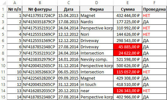
Необходимо сбросить форматирование ячеек и сделать так чтобы на всех таблицах планов выполнения работ были одинаковые форматы отображения данных. Формат ячеек для исходной таблицы должен быть закреплен за шаблоном, чтобы можно было сделать сброс и применять заданный стиль оформления в дальнейшем.

Чтобы выполнять такие задачи вручную можно попытаться облегчить процесс настройки множества опций форматирования для многих диапазонов ячеек на разных листах и рабочих книгах. Плюс к о всему можно ошибиться и применить несколько другие настройки форматирования.

Макросы Excel прекрасно справляются с форматированием ячеек на рабочих листах. Кроме того, делают это быстро и в полностью автоматическом режиме. Воспользуемся этими преимуществами и для решения данной задачи напишем свой код VBA-макроса. Он поможет нам быстро и безопасно сбрасывать форматы на исходный предварительно заданный в шаблоне главной таблицы.

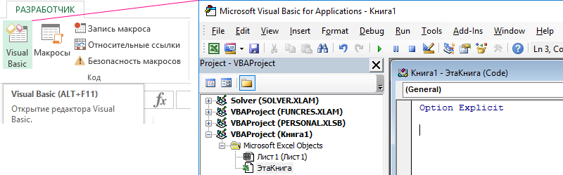
Чтобы написать свой код макроса откройте специальный VBA-редактор в Excel: «РАЗРАБОТЧИК»-«Код»-«Visual Basic» или нажмите комбинацию клавиш ALT+F11:

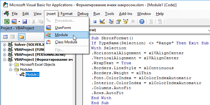
В редакторе создайте новый модуль выбрав инструмент «Insert»-«Module» и введите в него такой VBA-код макроса:

Sub SbrosFormat()
If TypeName(Selection) <> "Range" Then Exit Sub
With Selection
.HorizontalAlignment = xlVAlignCenter
.VerticalAlignment = xlVAlignCenter
.WrapText = True
.Borders.LineStyle = xlContinuous
.Borders.Weight = xlThin
.Font.ColorIndex = xlColorIndexAutomatic
.Interior.ColorIndex = xlColorIndexAutomatic
.Columns.AutoFit
.Rows.AutoFit
End With
End Sub


Теперь если нам нужно сбросить форматирование таблицы на исходный формат отображения ее данных, выделите диапазон ячеек A1:E20 и запустите макрос: «РАЗРАБОЧТИК»-«Код»-«Макросы»-«SbrosFormat»-«Выполнить». Результат работы макроса изображен ниже на рисунке:

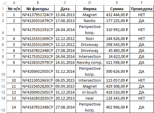
Таблица приобрела формат, который определен макросом. Таким образом код VBA нам позволяет сбросить любые изменения формата ячеек на предустановленный автором отчета.



Описание VBA-макроса для формата ячеек таблицы Excel

Первая инструкция в коде, проверяет выделены ли ячейки диапазоном. Если перед выполнением макроса выделил другой элемент листа, например, график, тогда макрос закрывается и дальнейшие инструкции выполняться не будут. В противные случаи будут форматироваться все выделенные ячейки по очереди в соответствии с определенными настройками форматирования:

1. Текст в значениях ячеек выравнивается по центру горизонтально и вертикально.
2. Включен построчный перенос текста.
3. Все границы ячеек получают черную обычной толщины непрерывную линию с черным цветом.
4. Сброс цвета шрифта на авто.
5. Удаляется любая заливка ячеек.
6. Ширина столбцов автоматически настраивается под текст в ячейках.
7. Автоматически настроить высоту строк по содержимому ячеек.

Модификация исходного кода макроса для форматирования

Если необходимо сделать так чтобы текст выравнивался не по центру относительно горизонтали, а по правую сторону ячейки, тогда измените константу xlHAlignCenter на xlHAlignRight. Она находиться в свойстве .HorizontalAlignment. Сделайте это следующим образом:

.HorizontalAlignment = xlHAlignRight.

Таким же образом можно выровнять текст по левую сторону изменив значение константы на xlHAlignLeft. Или можно выровнять положение текста по ширине ячейки используя константу xlHAlignJustify.

Чтобы макрос выравнивал текст в ячейках по вертикали к низу, измените строку кода, отвечающую за данную настройку форматирования. Измените константу, которая присваивается к свойству VerticalAlignment в следующий способ:

Если хотите выровнять текс к верху ячейки, тогда воспользуйтесь константой xlHAlignTop.

Если нужно применить для границ ячеек толстую и пунктирную линию в синем цвете, смодифицируйте инструкцию, отвечающую за формат линий:

.Borders.LineStyle = xlDash

.Borders.Color = vbBlue

.Borders.Weight = xlMedium

Описание настройки форматирования для линий границ ячеек. Мы будем получать разные дополнительные типы линий границ если для свойства LineStyle присваивать такие константы:

• xlDoshDot – применяется для рисования пунктирных линий в границах ячеек;
• xlDouble – рисует двойную линию;
• xlHairLine – рисует тонкую линию;
• xlThick – для рисования очень толстой линии.

Для настройки цвета линий Excel предлагает всего 8 констант для определенных цветов. Константы для настройки цвета линий границ для свойства Color:

• vbBlack – черный;
• vbWhite – белый;
• vbRed – красный;
• vbGreen –зеленый;
• vbBlue – синий;
• vbYellow – желтый;
• vbMagenta – алый;
• vbCyan – голубой.

Но при необходимости присвоить линиям границ другие цвета можно вместо константы для свойства Color записать функцию RGB(). Достаточно лишь в аргументе этой функции указать код цвета по шкале от 0 и до 255.

Если нужно применить толстую линию только для границ выделенного диапазона, тогда перед инструкцией End With добавьте следующую строку кода:

.BorderAround xlContinuous, xlMedium, vbBlack

Описание: В первом аргументе для метода BorderAround можно записать также другой стиль линии. Во втором – толщину линии, а в третьем – цвет. Константы, которые можно присвоить в качестве значений для этих аргументов можно использовать те же, которые мы использовали для свойств: LineStyle, Weight, Color.

Если нужно экспонировать первую строку для выделенного диапазона с помощью жирного и курсивного шрифта значений ячеек. А также заполнить ячейки первой строки заливкой с голубым цветом, тогда в самом конце кода макроса перед последней инструкцией End Sub следует добавить несколько строк с VBA-кодом:

.Rows(1).Font.Bold = True

.Rows(1).Font.Italic = True

.Rows(1).Interior.Color = vbCyan

Если хотите присвоить такой же формат для не только для первой строки, но и для первого столбца выделенного диапазона, тогда скопируйте и вставьте ниже эти 3 строчки кода. После в последних трех строках измените свойство Rows на Columns.

.Columns (1).Font.Bold = True

.Columns (1).Font.Italic = True

.Columns (1).Interior.Color = vbCyan

Если нужно задать особенный формат для экспонирования последней строки выделенного диапазона, тогда измените число 1 в аргументе свойства Rows на число всех выделенных строк .Rows.Count. Например, добавьте в конец кода еще такую строку:

.Rows(.Rows.Count).Font.Bold = True

Полная версия модифицированного кода макроса выглядит так:

Sub SbrosFormat()
If TypeName(Selection) <> "Range" Then Exit Sub
With Selection
.HorizontalAlignment = xlVAlignCenter
.VerticalAlignment = xlVAlignCenter
.WrapText = True
.Borders.LineStyle = xlDash
.Borders.Color = vbBlue
.Borders.Weight = xlMedium
.Font.ColorIndex = xlColorIndexAutomatic
.Interior.ColorIndex = xlColorIndexAutomatic
.Columns.AutoFit
.Rows.AutoFit
.BorderAround xlContinuous, xlMedium, vbBlack
.Rows(1).Font.Bold = True
.Rows(1).Font.Italic = True
.Rows(1).Interior.Color = vbCyan
.Columns(1).Font.Bold = True
.Columns(1).Font.Italic = True
.Columns(1).Interior.Color = vbCyan
.Rows(.Rows.Count).Font.Bold = True
End With
End Sub


Пример работы измененного кода VBA-макроса:

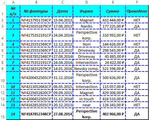
В данном примере вы ознакомились с базовыми возможностями форматирования с помощью VBA-макросов. Уверен, что теперь вы сможете самостоятельно найти практическое применение этим исходным кодам.