
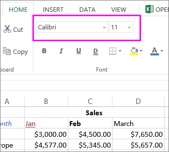
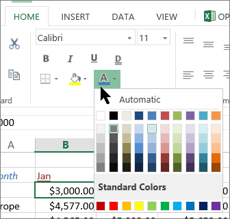
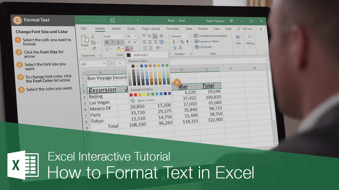
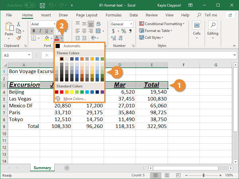
Change font style, size, color, or apply effects
Click Home and:
-
For a different font style, click the arrow next to the default font Calibri and pick the style you want.
-
To increase or decrease the font size, click the arrow next to the default size 11 and pick another text size.

-
To change the font color, click Font Color and pick a color.
-
To add a background color, click Fill Color next to Font Color.
-
To apply strikethrough, superscript, or subscript formatting, click the Dialog Box Launcher, and select an option under Effects.
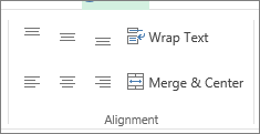
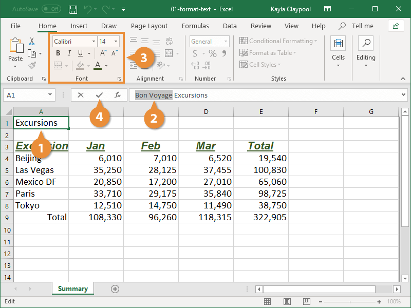
Change the text alignment
You can position the text within a cell so that it is centered, aligned left or right. If it’s a long line of text, you can apply Wrap Text so that all the text is visible.
Select the text that you want to align, and on the Home tab, pick the alignment option you want.
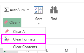
Clear formatting
If you change your mind after applying any formatting, to undo it, select the text, and on the Home tab, click Clear > Clear Formats.
Change font style, size, color, or apply effects
Click Home and:
-
For a different font style, click the arrow next to the default font Calibri and pick the style you want.
-
To increase or decrease the font size, click the arrow next to the default size 11 and pick another text size.
-
To change the font color, click Font Color and pick a color.
-
To add a background color, click Fill Color next to Font Color.
-
For boldface, italics, underline, double underline, and strikethrough, select the appropriate option under Font.

Change the text alignment
You can position the text within a cell so that it is centered, aligned left or right. If it’s a long line of text, you can apply Wrap Text so that all the text is visible.
Select the text that you want to align, and on the Home tab, pick the alignment option you want.
Clear formatting
If you change your mind after applying any formatting, to undo it, select the text, and on the Home tab, click Clear > Clear Formats.
Содержание
- Convert numbers into words
- Create the SpellNumber function to convert numbers to words
- Use the SpellNumber function in individual cells
- Save your SpellNumber function workbook
- Функция ТЕКСТ
- Общие сведения
- Скачивание образцов
- Другие доступные коды форматов
- Коды форматов по категориям
- Типичный сценарий
- Вопросы и ответы
Convert numbers into words
Excel doesn’t have a default function that displays numbers as English words in a worksheet, but you can add this capability by pasting the following SpellNumber function code into a VBA (Visual Basic for Applications) module. This function lets you convert dollar and cent amounts to words with a formula, so 22.50 would read as Twenty-Two Dollars and Fifty Cents. This can be very useful if you’re using Excel as a template to print checks.
If you want to convert numeric values to text format without displaying them as words, use the TEXT function instead.
Note: Microsoft provides programming examples for illustration only, without warranty either expressed or implied. This includes, but is not limited to, the implied warranties of merchantability or fitness for a particular purpose. This article assumes that you are familiar with the VBA programming language, and with the tools that are used to create and to debug procedures. Microsoft support engineers can help explain the functionality of a particular procedure. However, they will not modify these examples to provide added functionality, or construct procedures to meet your specific requirements.
Create the SpellNumber function to convert numbers to words
Use the keyboard shortcut, Alt + F11 to open the Visual Basic Editor (VBE).
Note: You can also access the Visual Basic Editor by showing the Developer tab in your ribbon.
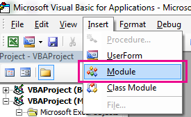
Click the Insert tab, and click Module.
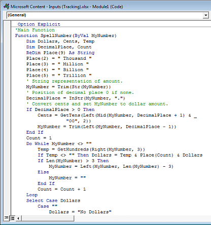
Copy the following lines of code.
Note: Known as a User Defined Function (UDF), this code automates the task of converting numbers to text throughout your worksheet.
Paste the lines of code into the Module1 (Code) box.
Press Alt + Q to return to Excel. The SpellNumber function is now ready to use.
Note: This function works only for the current workbook. To use this function in another workbook, you must repeat the steps to copy and paste the code in that workbook.
Use the SpellNumber function in individual cells
Type the formula =SpellNumber( A1) into the cell where you want to display a written number, where A1 is the cell containing the number you want to convert. You can also manually type the value like =SpellNumber(22.50).
Press Enter to confirm the formula.
Save your SpellNumber function workbook
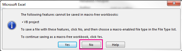
Excel cannot save a workbook with macro functions in the standard macro-free workbook format (.xlsx). If you click File > Save. A VB project dialog box opens. Click No.
You can save your file as an Excel Macro-Enabled Workbook (.xlsm) to keep your file in its current format.
Click File > Save As.
Click the Save as type drop-down menu, and select Excel Macro-Enabled Workbook.
Источник
Функция ТЕКСТ
С помощью функции ТЕКСТ можно изменить представление числа, применив к нему форматирование с кодами форматов. Это полезно в ситуации, когда нужно отобразить числа в удобочитаемом виде либо объединить их с текстом или символами.
Примечание: Функция ТЕКСТ преобразует числа в текст, что может затруднить их использование в дальнейших вычислениях. Рекомендуем сохранить исходное значение в одной ячейке, а функцию ТЕКСТ использовать в другой. Затем, если потребуется создать другие формулы, всегда ссылайтесь на исходное значение, а не на результат функции ТЕКСТ.
Аргументы функции ТЕКСТ описаны ниже.
Числовое значение, которое нужно преобразовать в текст.
Текстовая строка, определяющая формат, который требуется применить к указанному значению.
Общие сведения
Самая простая функция ТЕКСТ означает следующее:
=ТЕКСТ(значение, которое нужно отформатировать; «код формата, который требуется применить»)
Ниже приведены популярные примеры, которые вы можете скопировать прямо в Excel, чтобы поэкспериментировать самостоятельно. Обратите внимание: коды форматов заключены в кавычки.
Денежный формат с разделителем групп разрядов и двумя разрядами дробной части, например: 1 234,57 ₽. Обратите внимание: Excel округляет значение до двух разрядов дробной части.
Сегодняшняя дата в формате ДД/ММ/ГГ, например: 14.03.12
Сегодняшний день недели, например: понедельник
Текущее время, например: 13:29
Процентный формат, например: 28,5 %
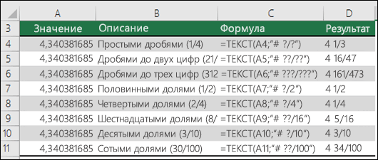
Дробный формат, например: 4 1/3
Дробный формат, например: 1/3 Обратите внимание: функция СЖПРОБЕЛЫ используется для удаления начального пробела перед дробной частью.
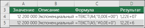
Экспоненциальное представление, например: 1,22E+07
Добавление нулей в начале, например: 0001234
Пользовательский формат (широта или долгота), например: 12° 34′ 56»
Примечание: Функцию ТЕКСТ можно использовать для изменения форматирования, но это не единственный способ. Чтобы изменить форматирование без формулы, нажмите клавиши CTRL+1 (на компьютере Mac —  +1), а затем в диалоговом окне Формат ячеек на вкладке Число выберите нужный формат.
Скачивание образцов
Предлагаем скачать книгу, в которой содержатся все примеры применения функции ТЕКСТ из этой статьи и несколько других. Вы можете воспользоваться ими или создать собственные коды форматов для функции ТЕКСТ.
Другие доступные коды форматов
Просмотреть другие доступные коды форматов можно в диалоговом окне Формат ячеек.
Нажмите клавиши CTRL+1 (на компьютере Mac — +1), чтобы открыть диалоговое окно Формат ячеек.
На вкладке Число выберите нужный формат.
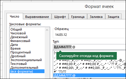
Выберите пункт (все форматы).
Нужный код формата будет показан в поле Тип. В этом случае выделите всё содержимое поля Тип, кроме точки с запятой (;) и символа @. В примере ниже выделен и скопирован только код ДД.ММ.ГГГГ.
Нажмите клавиши CTRL+C, чтобы скопировать код формата, а затем — кнопку Отмена, чтобы закрыть диалоговое окно Формат ячеек.
Теперь осталось нажать клавиши CTRL+V, чтобы вставить код формата в функцию ТЕКСТ. Пример: =ТЕКСТ(B2;» ДД.ММ.ГГГГ«). Обязательно заключите скопированный код формата в кавычки («код формата»), иначе в Excel появится сообщение об ошибке.
 «Ячейки» > «Число» > «Другое» для получения строк формата.» loading=»lazy»>
Коды форматов по категориям
В примерах ниже показано, как применить различные числовые форматы к значениям следующим способом: открыть диалоговое окно Формат ячеек, выбрать пункт (все форматы) и скопировать нужный код формата в формулу с функцией ТЕКСТ.
Почему программа Excel удаляет нули в начале?
Excel воспринимает последовательность цифр, введенную в ячейку, как число, а не как цифровой код, например артикул или номер SKU. Чтобы сохранить нули в начале последовательностей цифр, перед вставкой или вводом значений примените к соответствующему диапазону ячеек текстовый формат. Выделите столбец или диапазон, в который нужно поместить значения, нажмите клавиши CTRL+1, чтобы открыть диалоговое окно Формат ячеек, и выберите на вкладке Число пункт Текстовый. Теперь программа Excel не будет удалять нули в начале.
Если вы уже ввели данные и Excel удалил начальные нули, вы можете снова добавить их с помощью функции ТЕКСТ. Создайте ссылку на верхнюю ячейку со значениями и используйте формат =ТЕКСТ(значение;»00000″), где число нулей представляет нужное количество символов. Затем скопируйте функцию и примените ее к остальной части диапазона.
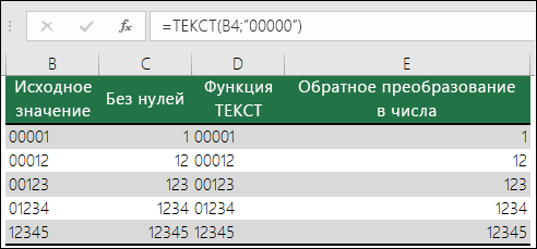
Если по какой-либо причине потребуется преобразовать текстовые значения обратно в числа, можно умножить их на 1 (например: =D4*1) или воспользоваться двойным унарным оператором (—), например: =—D4.
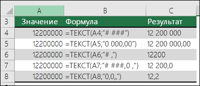
В Excel группы разрядов разделяются пробелом, если код формата содержит пробел, окруженный знаками номера (#) или нулями. Например, если используется код формата «# ###», число 12200000 отображается как 12 200 000.
Пробел после заполнителя цифры задает деление числа на 1000. Например, если используется код формата «# ###,0 «, число 12200000 отображается в Excel как 12 200,0.
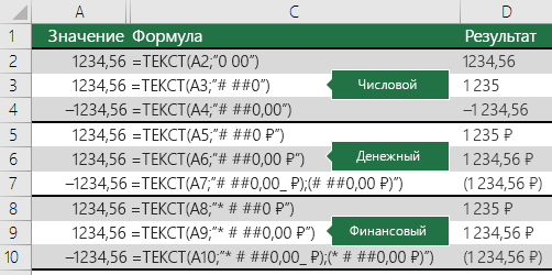
Разделитель групп разрядов зависит от региональных параметров. Для России это пробел, но в других странах и регионах может использоваться запятая или точка.
Разделитель групп разрядов можно применять в числовых, денежных и финансовых форматах.
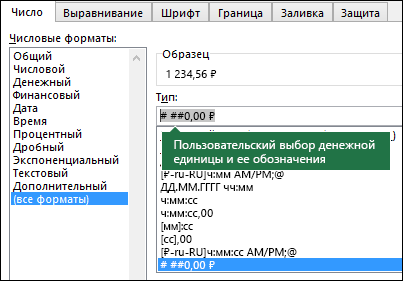
Ниже показаны примеры стандартных числовых (только с разделителем групп разрядов и десятичными знаками), денежных и финансовых форматов. В денежном формате можно добавить нужное обозначение денежной единицы, и значения будут выровнены по нему. В финансовом формате символ рубля располагается в ячейке справа от значения (если выбрать обозначение доллара США, то эти символы будут выровнены по левому краю ячеек, а значения — по правому). Обратите внимание на разницу между кодами денежных и финансовых форматов: в финансовых форматах для отделения символа денежной единицы от значения используется звездочка (*).
Чтобы получить код формата для определенной денежной единицы, сначала нажмите клавиши CTRL+1 (на компьютере Mac — +1) и выберите нужный формат, а затем в раскрывающемся списке Обозначение выберите символ.
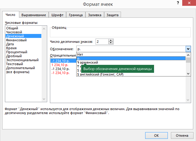
После этого в разделе Числовые форматы слева выберите пункт (все форматы) и скопируйте код формата вместе с обозначением денежной единицы.
Примечание: Функция ТЕКСТ не поддерживает форматирование с помощью цвета. Если скопировать в диалоговом окне «Формат ячеек» код формата, в котором используется цвет, например «# ##0,00 ₽; [Красный]# ##0,00 ₽», то функция ТЕКСТ воспримет его, но цвет отображаться не будет.
Способ отображения дат можно изменять, используя сочетания символов «Д» (для дня), «М» (для месяца) и «Г» (для года).
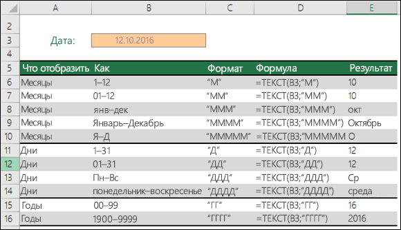
В функции ТЕКСТ коды форматов используются без учета регистра, поэтому допустимы символы «М» и «м», «Д» и «д», «Г» и «г».

Если вы предоставляете общий доступ к файлам и отчетам Excel пользователям из разных стран, скорее всего, потребуется, чтобы они были на разных языках. Минда Триси (Mynda Treacy), Excel MVP, предлагает отличное решение этой задачи в своей статье Отображение дат Excel на разных языках (на английском). В ней также есть пример книги, который вы можете скачать.
Способ отображения времени можно изменить с помощью сочетаний символов «Ч» (для часов), «М» (для минут) и «С» (для секунд). Кроме того, для представления времени в 12-часовом формате можно использовать символы «AM/PM».
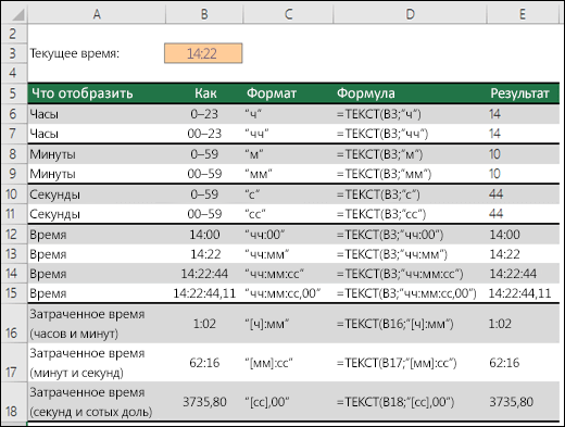
Если не указывать символы «AM/PM», время будет отображаться в 24-часовом формате.
В функции ТЕКСТ коды форматов используются без учета регистра, поэтому допустимы символы «Ч» и «ч», «М» и «м», «С» и «с», «AM/PM» и «am/pm».
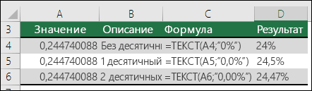
Для отображения десятичных значений можно использовать процентные (%) форматы.
Десятичные числа можно отображать в виде дробей, используя коды форматов вида «?/?».
Экспоненциальное представление — это способ отображения значения в виде десятичного числа от 1 до 10, умноженного на 10 в некоторой степени. Этот формат часто используется для краткого отображения больших чисел.
В Excel доступны четыре дополнительных формата:
«Почтовый индекс» («00000»);
«Индекс + 4» («00000-0000»);
«Табельный номер» («000-00-0000»).
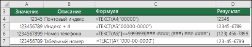
Дополнительные форматы зависят от региональных параметров. Если же дополнительные форматы недоступны для вашего региона или не подходят для ваших нужд, вы можете создать собственный формат, выбрав в диалоговом окне Формат ячеек пункт (все форматы).
Типичный сценарий
Функция ТЕКСТ редко используется сама по себе, а чаще применяется в сочетании с чем-то еще. Предположим, что вы хотите объединить текст и числовое значение, например, чтобы получить строку «Отчет напечатан 14.03.12» или «Еженедельный доход: 66 348,72 ₽». Такие строки можно ввести вручную, но суть в том, что Excel может сделать это за вас. К сожалению, при объединении текста и форматированных чисел, например дат, значений времени, денежных сумм и т. п., Excel убирает форматирование, так как неизвестно, в каком виде нужно их отобразить. Здесь пригодится функция ТЕКСТ, ведь с ее помощью можно принудительно отформатировать числа, задав нужный код формата, например «ДД.ММ.ГГГГ» для дат.
В примере ниже показано, что происходит, если попытаться объединить текст и число, не применяя функцию ТЕКСТ. Мы используем амперсанд ( &) для сцепления текстовой строки, пробела (» «) и значения: =A2&» «&B2.
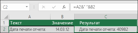
Вы видите, что значение даты, взятое из ячейки B2, не отформатировано. В следующем примере показано, как применить нужное форматирование с помощью функции ТЕКСТ.
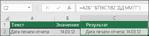
Вот обновленная формула:
ячейка C2: =A2&» «&ТЕКСТ(B2;»дд.мм.гггг») — формат даты.
Вопросы и ответы
К сожалению, это невозможно сделать с помощью функции ТЕКСТ. Для этого нужно использовать код Visual Basic для приложений (VBA). В следующей статье описано, как это сделать: Как преобразовать числовое значение в слова в Excel
Да, вы можете использовать функции ПРОПИСН, СТРОЧН и ПРОПНАЧ. Например, формула =ПРОПИСН(«привет») возвращает результат «ПРИВЕТ».
Да, но для этого необходимо выполнить несколько действий. Сначала выделите нужные ячейки и нажмите клавиши CTRL+1, чтобы открыть диалоговое окно Формат ячеек. Затем на вкладке Выравнивание в разделе «Отображение» установите флажок Переносить по словам. После этого добавьте в функцию ТЕКСТ код ASCII СИМВОЛ(10) там, где нужен разрыв строки. Вам может потребоваться настроить ширину столбца, чтобы добиться нужного выравнивания.

В этом примере использована формула =»Сегодня: «&СИМВОЛ(10)&ТЕКСТ(СЕГОДНЯ();»ДД.ММ.ГГ»).
Это экспоненциальное представление числа. Excel автоматически приводит к такому виду числа длиной более 12 цифр, если к ячейкам применен формат Общий, и числа длиннее 15 цифр, если выбран формат Числовой. Если вы вводите длинные цифровые строки, но не хотите, чтобы они отображались в таком виде, то сначала примените к соответствующим ячейкам формат Текстовый.
Если вы предоставляете общий доступ к файлам и отчетам Excel пользователям из разных стран, скорее всего, потребуется, чтобы они были на разных языках. Минда Триси (Mynda Treacy), Excel MVP, предлагает отличное решение этой задачи в своей статье Отображение дат Excel на разных языках (на английском). В ней также есть пример книги, который вы можете скачать.
Источник
How to Format Text in Excel?
Formatting text in Excel includes color, font name, font size, alignment, font appearance in bold, underline, italic, background color of the font cell, etc.
Table of contents
- How to Format Text in Excel?
- #1 Text Name
- #2 Font Size
- #3 Text Appearance
- #4 Text Color
- #5 Text Alignment
- #6 Text Orientation
- #7 Conditional Text Formatting
- #1 – Highlight Specific Value
- #2 – Highlight Duplicate Value
- #3 – Highlight Unique Value
- Things to Remember
- Recommended Articles
You can download this Formatting Text Excel Template here – Formatting Text Excel Template
#1 Text Name
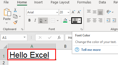
We can format the text font from default to any other available fonts in Excel. Likewise, we can insert any text value in any of the cells.
Under the “Home” tab, we can see so many formatting options available.
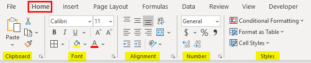
Formatting has been categorized into six groups: “Clipboard,” “Font,” “Alignment,” “Number,” and “Styles.”
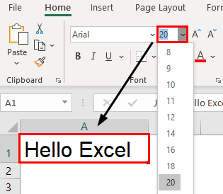
In this, we are formatting the font of cell value A1, “Hello Excel.” For this, under the “Font” category, click on the “Font Name” drop-down list and select the font name as per wish.
We hover over one of the font names above. We can see the quick preview in cell A1. If you are satisfied with the font style, click on the name to fix the font name for the selected cell value.
#2 Font Size
Similarly, we can also format the font size of the text in a cell. Just type the font size in numbers next to the font name option.
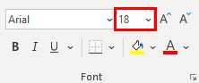
Enter the font size in numbers to see the impact.
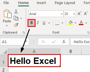
#3 Text Appearance
We can modify the default view of the text value. For example, we can make the text value look bold, italic, and underlined. Look at font size and name options. We can see all these three options.
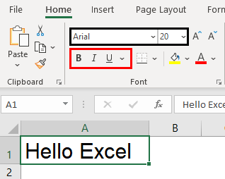
As per the format, we can apply formatting to text value.
- We have applied the “Bold” formatting using the Ctrl + B shortcut excel keyAn Excel shortcut is a technique of performing a manual task in a quicker way.read more.
![]()
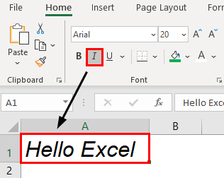
- To apply “Italic” formatting, use the Ctrl + I shortcut key.
![]()
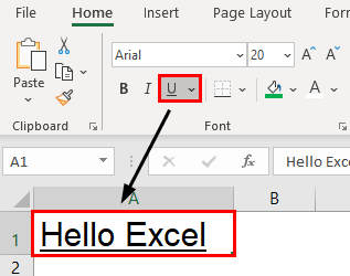
- To apply “Underline” formatting, use the Ctrl + U shortcut key.
![]()
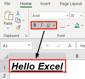
- The below image shows a combination of all the above three options.
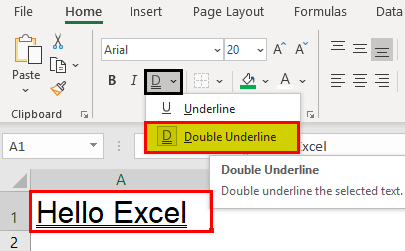
- If we want to apply a double underline, click on the drop-down list of underline options and choose “Double Underline.”
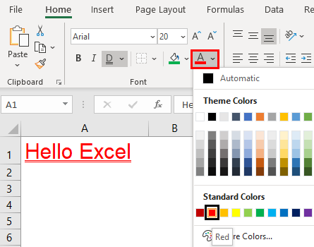
#4 Text Color
We can format the default font color (black) of text to any colors available.
- Click on the drop-down list of the “Font Color” option and change as per choice.
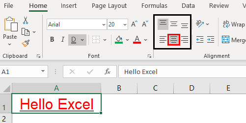
#5 Text Alignment
We can format the alignment of the Excel text under the “Alignment” group.
- We can do a left alignment, right alignment, middle alignment, top alignment, and bottom alignment.
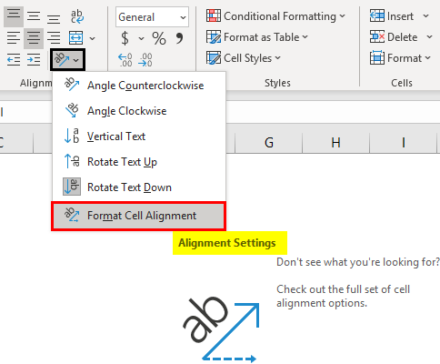
#6 Text Orientation
The important thing under “Alignment” is the “Orientation” of the text value.
Under “Orientation,” we can rotate text values diagonally or vertically.
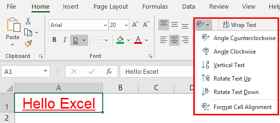
- Angle Counterclockwise
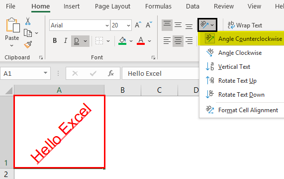
- Angle Clockwise
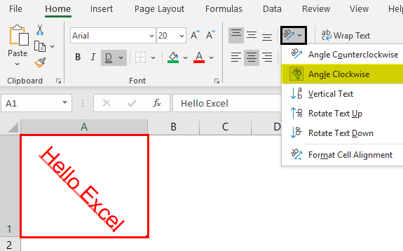
- Vertical Text

- Rotate Text Up

- Rotate Text Down
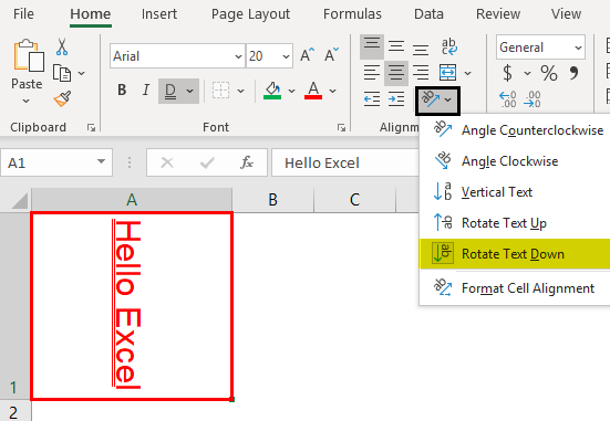
- Under “Format Cell Alignment, we have many options. Click on this option and experiment with some techniques to see the impact.
#7 Conditional Text Formatting
Let us see how to apply conditional formattingConditional formatting is a technique in Excel that allows us to format cells in a worksheet based on certain conditions. It can be found in the styles section of the Home tab.read more to text in Excel.
We have learned some of the basic text formatting techniques. How about the idea of formatting only a specific set of values from the group? If we want to find only duplicate values or find unique values.
These are possible through the conditional formatting technique.
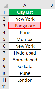
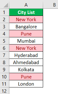
For example, look at the below list of cities.
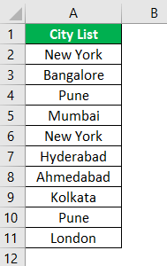
From this list, let us learn some formatting techniques.
#1 – Highlight Specific Value
If we want to highlight only the specific city name, we can only highlight specific city names. For example, assume we want to highlight the city “Bangalore,” then select the data and go to conditional formatting.
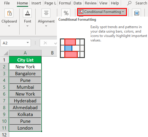
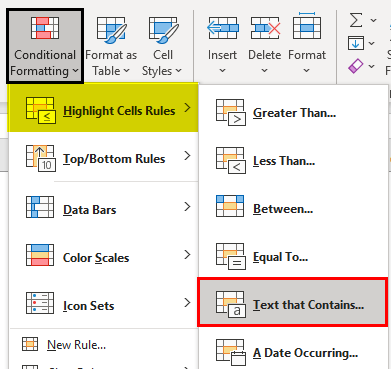
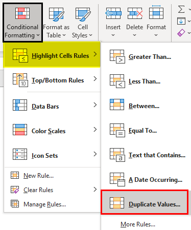
Click on the drop-down list in excelA drop-down list in excel is a pre-defined list of inputs that allows users to select an option.read more of “Conditional Formatting” >>> “Highlight cells Rules” >>> “Text that Contains.”
Now, we will see the below window.
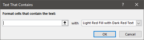
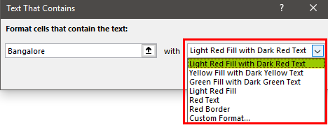
Next, we must enter the text value that we need to highlight.
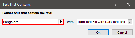
Now from the drop-down list, we must choose the formatting style.
Click on “OK.” Consequently, it will highlight only the supplied text value.
#2 – Highlight Duplicate Value
To highlight duplicate values in excelHighlight Cells Rule, which is available under Conditional Formatting under the Home menu tab, can be used to highlight duplicate values in the selected dataset, whether it is a column or row of a table.read more, follow the below path.
“Conditional Formatting” >>> “Highlight cells Rules” >>> “Duplicate Values.”
Again from the below window, we must select the formatting style.
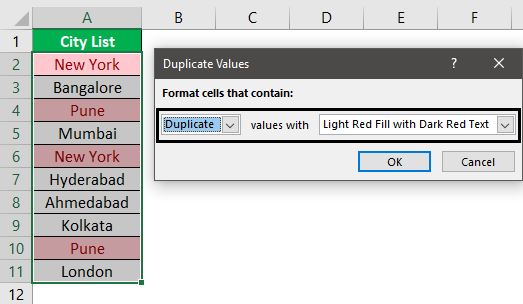
As a result, it will highlight only the text values that appear more than once.
#3 – Highlight Unique Value
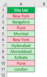
Like how we have highlighted duplicate values similarly, we can highlight all the unique values, i.e., text value that appears only once. Then, the formatting window chooses the “Unique” value option from the duplicate values.
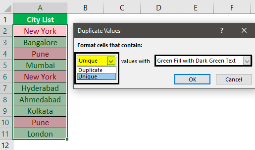
It will highlight only the unique values.
Things to Remember
- We must learn shortcut keys to format text values in Excel quickly.
- We can use conditional formatting to format some text values based on certain conditions.
Recommended Articles
This article is a guide to formatting text in Excel. We discuss formatting text using text name, font size, appearance, color, etc., with practical examples and downloadable Excel templates. You may learn more about Excel from the following articles: –
- Conditional Formatting in Dates
- Conditional Formatting along with Formulas
- Combine Text From Two Or More Cells

Excel Formatting Text (Table of Contents)
- Introduction to Formatting Text in Excel
- Text Formatting Tools
Introduction to Formatting Text in Excel
Excel has a wide range of variety for text formatting, which can make your results, dashboards, spreadsheets, an analysis that you do on day to day basis look fancier and attractive at the same time. Text formatting in Excel works in the same way as it does in other Microsoft tools such as Word and PowerPoint. This includes changing Font, Font Size, Font Color, Font Attribute (Such as making text, Bold, Italic, Underlined, etc.), text alignment, background color change, etc. This article will cover these text formatting tools in Excel along with examples for better understanding. Basically, all text formatting can be divided into two major groups, which are Font and Alignment. Each group has a variety of options using which we can format the text values and has its own relevance. e.g. within Font, you can have all the options associated with text fonts.
Please find attached is the screenshot for your reference:

Text Formatting Tools
All these text formatting tools are placed under the home tab. I am not considering the Clipboard in it because most of its part contains the cut, copy, paste, and Format Painter. Let’s start with Font and its options.
You can download this Formatting Text Excel Template here – Formatting Text Excel Template
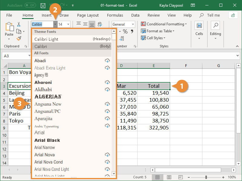
1. Text Font
The first thing that comes into the picture when we talk about text formatting is Text Font. The default text font in Excel is set as Calibri (Body). However, it can be changed to any of the variety available in the fonts section.
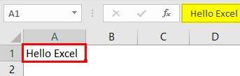
Let’s add some text under cell A1 of the Excel sheet.

As can be seen through the screenshot above, we have added as text “Hello World!” under cell A1 of the Excel sheet.
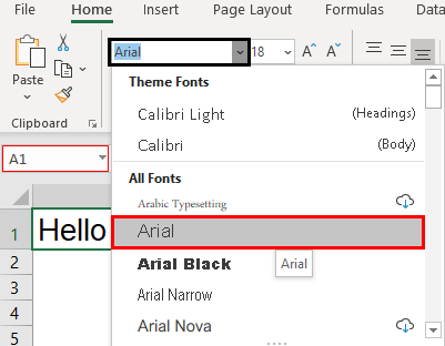
Navigate towards the Font section, where the default value is set as Calibri. Click on the dropdown menu, and you can see multiple fonts in which you can use for the text in cell A1. Choose anyone of your choice; I will use the Arial Black.

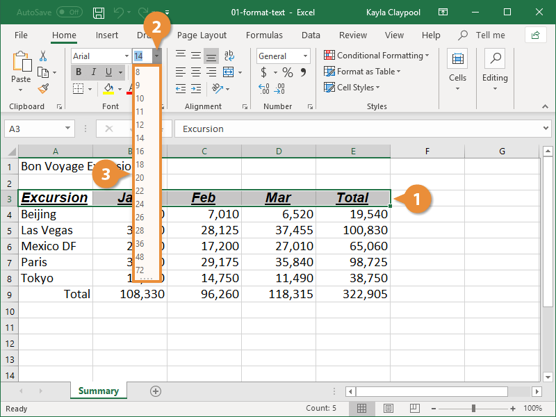
Now, we will try to change the font size.
Select the cell containing text (A1 in our example) and navigate towards the Font Size dropdown placed besides the Font option. Click on the dropdown, and you can see different font sizes starting from as low as 8. I will change the font size to 16. Please see the screenshot below for your reference.

You can also increase or decrease the font size using the Increase Font Size and Decrease Font Size buttons, which are placed right beside the Font Size dropdown. See the screenshot below:

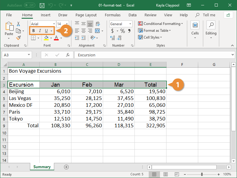
The next part comes when we have to change the text appearance. This covers the Bold, Italic, underlined text as well as coloring the text and/or cell containing the same.
Select the cell containing text and click on the bold button. It will make the text appear in bold. You can also achieve this by hitting Ctrl + B keys.

Select the cell and click on the Italic button that converts the text into Italic font. This can be achieved through a keyboard shortcut Ctrl + I.

You can underline the text by using the Underline button that is placed besides the Italic button; the keyboard shortcut to achieve this result is Ctrl + U. There is one more option for the underlined section, and it is Double Underline. It adds a double underline to the current cell containing text. See the screenshot below for better visualization of these two options.

We also have an option to change the text color for a given text. This option is placed under the Font section in your excel ribbon. You can simply click on the change color dropdown and see different colors to add for the current text value. See the screenshot below for your reference:

This is how we can format the text using the Font Group. Now we will move towards the second group called Alignment.
2. Text Alignment
This part also plays an important role in text formatting. We have several alignment options available under this Group. We will see that one by one. Text alignment is of 6 types in total. The first three are Top Align, Middle Align, and Bottom Align. These are placed at the top most tier under the Alignment group.

Exactly below to these three, there are three more alignment options. Align Left, Center and Align Right. They are placed in the second tier of the options under the Alignment group.

The third part that gets covered under the Alignment group is the Text Rotation option. This option has different text rotation options available, allowing you to rotate the text with angles (clockwise)and vertically (up and Down). This feature is rarely used though sometimes it is really helpful when you want to do something different with the headings of your reports.

Forth thing that gets covered under the Alignment section is the indentation. Most of us fail to recognize when to add or decrease an indentation. However, you don’t need to keep it in your mind. Excel has Increase Indent and Decrease Indent option that helps you either increase or decrease the indent in your current text.

The fifth and last thing that comes under alignment is Wrap Text and Merge& Center option. Well, these two are the most commonly used alignment operations in Excel. Wrap Text shows text in one single cell even if that text goes beyond the cell boundaries. On the other hand, Merge & Center merges the data across the multiple cells and then makes a centered alignment for the merged text. If you click on Merge & Center button again, it removes the effect; however, the text gets filled in the left most cell or a cell under which it has actually been entered.

The above screenshot emphasizes the use of Wrap Text. The actual text under A1 is beyond the cell boundary. However, with it having wrapped, it is under the cell boundary.

This screenshot emphasizes the use of Merge and Center. Instead of wrapping the text under same cell, we have tried it to merge across three cells A3:C3 and it looks nicer than before. This is how Merge & Center works.
This is how we can format the text under Excel. Now let’s wrap things up with some points to be remembered about Text Formatting in Excel.
Things to Remember
- Font and Alignment covers most of the Text Formatting options under Excel
- Some of the users also consider Conditional Formatting as a part of Text Formatting. It sometimes can be used to format the text. However, it is not dedicated to text formatting (We can also use conditional formatting on numbers).
- You can use the Format Painter option under Clipboard to copy the text format and apply it to some other text in some other cell or sheet.
Recommended Articles
This has been a guide to Formatting Text in Excel. Here we discuss How to use Formatting Text in Excel along with practical examples and a downloadable excel template. You can also go through our other suggested articles –
- VBA Conditional Formatting
- Excel Text with Formula
- Search For Text in Excel
- Count Cells with Text in Excel
A quick way to change the appearance of your spreadsheet is to change the font of the text. A font is a set of letters, numbers, and punctuation symbols designed around a shared appearance. A font will have variations for size and styles, such as bold and italics.
Change Fonts
Changing the font is a quick and simple way to enhance the appearance of your spreadsheet.
- Select the cells you want to format.
- Click the Font list arrow on the Home tab.
When text is selected in a cell, you can also click the Font list arrow on the Mini Toolbar.
- Select the font you want to use.

Apply Bold, Italic, or an Underline
In addition to changing the font type, you can amplify your project using other features in the Font group such as Bold, Italic, or Underline.
- Select the text you want to format.
- Click the Bold, Italic, or Underline buttons on the Home tab.
- To bold, press Ctrl + B.
- To italicize, press Ctrl + I.
- To underline, press Ctrl + U.
Click the Dialog Box Launcher in the Font group to see additional font formatting options. From the dialog box, you can change the underline style and add effects.
Change Font Size
Changing the font size can help differentiate between titles, headers, and body text.
- Select the cells you want to format.
- Click the Font Size list arrow.
Font size is measured in points (pt.) that are 1/72 of an inch. The larger the number of points, the larger the font.
- Select the font size you want.
Click the Increase Font Size or Decrease Font Size buttons on the Home tab to adjust the font size.
Change Font Color
Changing font color makes text stand out against the white background of the spreadsheet.
- Select the cells you want to format.
- Click the Font Color list arrow.
When text is selected in a cell, you can also click the Font Color list arrow on the Mini Toolbar.
- Select a new color.
Format Part of a Cell
- Select the cell you want to format.
- In the formula bar, select the text you want to format.
- Select the text formatting you want to use.
- Press Enter.

FREE Quick Reference
Click to Download
Free to distribute with our compliments; we hope you will consider our paid training.
Transcript
In this lesson we’ll look at how to apply local formatting to individual characters and words.
Let’s take a look.
Sometimes you need to apply formatting to only a few characters or words. It doesn’t work to select a cell and apply the formatting, because that will affect all of the content in the cell.
There are two ways to apply this kind of formatting. The first way is to select a cell and apply formatting in the formula bar. Start by selecting the text you want to format and select the format you like.
This works fine, but the formula bar won’t show any formatting, so you’ll want to keep an eye on the cell itself which will display all formatting changes.
When formatting just part of a cell, you can change the font, color, and size of text. You can also apply bold, italic, and underline styles.
The other way to apply formatting to individual characters is to double-click the cell, or press F2 to enable edit mode. In edit mode you can select text, apply formatting, and see the result, all in one place.
After you select the text in a cell, Excel will faintly display a small menu of formatting options. To access this menu, just hover over it with your mouse.
Be careful when you apply formatting to a cell that you’ve made character-level changes to; it can be tricky to keep these local changes intact. Excel does a pretty good job protecting local formatting in cells, but it can be lost easily when you apply certain formatting.
For example, if you apply a color to a cell, it will override any local color changes you’ve made.
In a similar way, applying a font to a cell that already has more than one font applied will remove all local font changes and reset the cell to the new font.

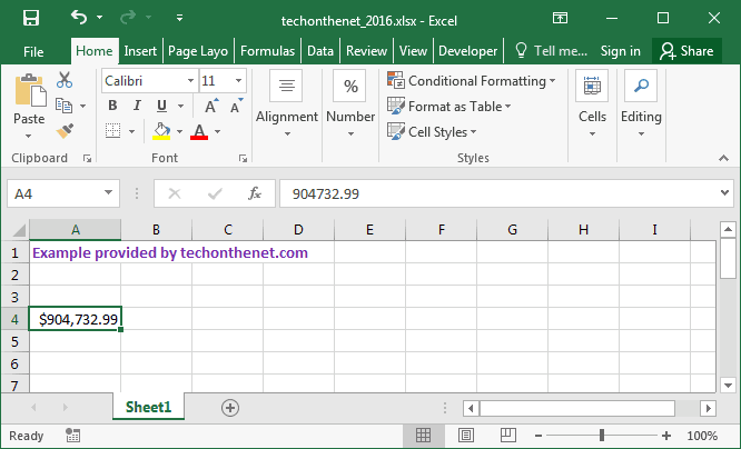
This Excel tutorial explains how to format the display of a cell’s text in Excel 2016 such as numbers, dates, etc (with screenshots and step-by-step instructions).
Question: How do I format how the text displays in a cell in Microsoft Excel 2016?
Answer: Select the cells that you wish to format.
Right-click and then select «Format Cells» from the popup menu.
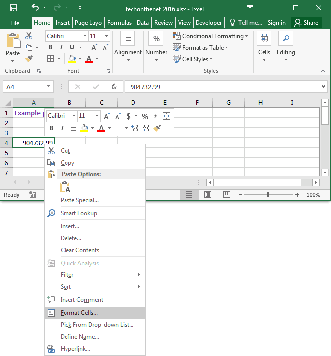
When the Format Cells window appears, select the Number tab. In the Category listbox, select your format. A sample of your text will appear on the right portion of the window based on the format that you’ve selected. Click the OK button when you are done.
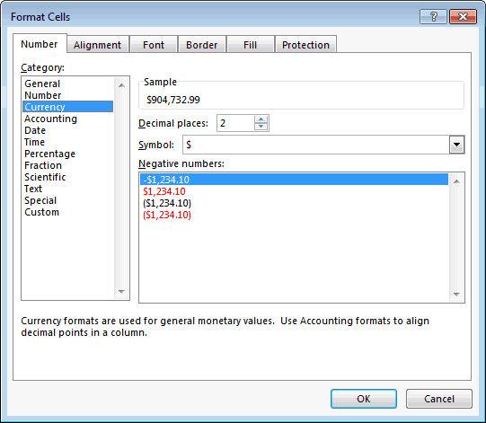
In this example, we’ve chosen to format the content of the cells as a currency number with 2 decimal places.
Skip to content
-
Check Also Extract Substring Between Parenthesis In Excel
-
Check Also Count Number Of Users Who Are Active In An Excel Workbook
-
Check Also VBA To Open Latest Excel Workbook
-
Check Also Print Cell Height And Cell Width Of A Cell In Excel
-
Check Also Delete Non Numeric Values From Numeric Field In Excel
-
Check Also Create Rows From Column In Excel
-
Check Also Sum Numbers Separated By Symbol In Excel
-
Check Also Sort Comma Separated Values Within A Cell In Excel
The post demonstrates how to format individual character/word in a sentence to a different format as shown in the pic below.

Sometimes we have a long paragraph or text in which we want to highlight some important things in a visually appealing way and also do not want to delete other remaining parts.
As you could see in the pic above, all the three words in a sentence are having a different font style or format; we could easily format different characters with different colors, different font style and different font size.
We will see below how we could apply different formats to different characters/words in excel.
Step 1
Select the first part i.e. “How” and change the font style to bold and change the font type to Arial Black in the home tab as shown in the fig below

Step 2
Now select a different text i.e. “are” and change the font style to italic and font type to Broadway as shown in the pic below.

And likewise you could choose different format for different words/character in excel.
I have selected the font type of “you” to Brush Script MT and changed the font color to Red.
Also, if you want you can format each individual character in a text in excel to a different format style.
Hope this helped.
Random Posts
-

-
-
Create Checklist In Excel
Let’s see how to create a checklist in excel to know the current status of the action items. Below checklist […]
-


