
Conditional formatting is a fantastic way to quickly visualize data in a spreadsheet. With conditional formatting, you can do things like highlight dates in the next 30 days, flag data entry problems, highlight rows that contain top customers, show duplicates, and more.
Excel ships with a large number of «presets» that make it easy to create new rules without formulas. However, you can also create rules with your own custom formulas. By using your own formula, you take over the condition that triggers a rule and can apply exactly the logic you need. Formulas give you maximum power and flexibility.
For example, using the «Equal to» preset, it’s easy to highlight cells equal to «apple».
But what if you want to highlight cells equal to «apple» or «kiwi» or «lime»? Sure, you can create a rule for each value, but that’s a lot of trouble. Instead, you can simply use one rule based on a formula with the OR function:

Here’s the result of the rule applied to the range B4:F8 in this spreadsheet:

Here’s the exact formula used:
=OR(B4="apple",B4="kiwi",B4="lime")
Quick start
You can create a formula-based conditional formatting rule in four easy steps:
1. Select the cells you want to format.

2. Create a conditional formatting rule, and select the Formula option

3. Enter a formula that returns TRUE or FALSE.

4. Set formatting options and save the rule.

The ISODD function only returns TRUE for odd numbers, triggering the rule:

Video: How to apply conditional formatting with a formula
Formula logic
Formulas that apply conditional formatting must return TRUE or FALSE, or numeric equivalents. Here are some examples:
=ISODD(A1)
=ISNUMBER(A1)
=A1>100
=AND(A1>100,B1<50)
=OR(F1="MN",F1="WI")
The above formulas all return TRUE or FALSE, so they work perfectly as a trigger for conditional formatting.
When conditional formatting is applied to a range of cells, enter cell references with respect to the first row and column in the selection (i.e. the upper-left cell). The trick to understanding how conditional formatting formulas work is to visualize the same formula being applied to each cell in the selection, with cell references updated as usual. Imagine that you entered the formula in the upper-left cell of the selection, and then copied the formula across the entire selection. If you struggle with this, see the section on Dummy Formulas below.
Formula Examples
Below are examples of custom formulas you can use to apply conditional formatting. Some of these examples can be created using Excel’s built-in presets for highlighting cells, but custom formulas can go far beyond presets, as you can see below.
Highlight orders from Texas
To highlight rows that represent orders from Texas (abbreviated TX), use a formula that locks the reference to column F:
=$F5="TX"

For more details, see this article: Highlight rows with conditional formatting.
Video: How to highlight rows with conditional formatting
Highlight dates in the next 30 days
To highlight dates occurring in the next 30 days, we need a formula that (1) makes sure dates are in the future and (2) makes sure dates are 30 days or less from today. One way to do this is to use the AND function together with the NOW function like this:
=AND(B4>NOW(),B4<=(NOW()+30))
With a current date of August 18, 2016, the conditional formatting highlights dates as follows:

The NOW function returns the current date and time. For details about how this formula, works, see this article: Highlight dates in the next N days.
Highlight column differences
Given two columns that contain similar information, you can use conditional formatting to spot subtle differences. The formula used to trigger the formatting below is:
=$B4<>$C4

See also: a version of this formula that uses the EXACT function to do a case-sensitive comparison.
Highlight missing values
To highlight values in one list that are missing from another, you can use a formula based on the COUNTIF function:
=COUNTIF(list,B5)=0

This formula simply checks each value in List A against values in the named range «list» (D5:D10). When the count is zero, the formula returns TRUE and triggers the rule, which highlights values in List A that are missing from List B.
Video: How to find missing values with COUNTIF
Highlight properties with 3+ bedrooms under $350k
To find properties in this list that have at least 3 bedrooms but are less than $300,000, you can use a formula based on the AND function:
=AND($C5<350000,$D5>=3)
The dollar signs ($) lock the reference to columns C and D, and the AND function is used to make sure both conditions are TRUE. In rows where the AND function returns TRUE, the conditional formatting is applied:

Highlight top values (dynamic example)
Although Excel has presets for «top values», this example shows how to do the same thing with a formula, and how formulas can be more flexible. By using a formula, we can make the worksheet interactive — when the value in F2 is updated, the rule instantly responds and highlights new values.

The formula used for this rule is:
=B4>=LARGE(data,input)
Where «data» is the named range B4:G11, and «input» is the named range F2. This page has details and a full explanation.
Gantt charts
Believe it or not, you can even use formulas to create simple Gantt charts with conditional formatting like this:

This worksheet uses two rules, one for the bars, and one for the weekend shading:
=AND(D$4>=$B5,D$4<=$C5) // bars
=WEEKDAY(D$4,2)>5 // weekends
This article explains the formula for bars, and this article explains the formula for weekend shading.
Simple search box
One cool trick you can do with conditional formatting is to build a simple search box. In this example, a rule highlights cells in column B that contain text typed in cell F2:

The formula used is:
=ISNUMBER(SEARCH($F$2,B2))
For more details and a full explanation, see:
- Article: How to highlight cells that contain specific text
- Article: How to highlight rows that contain specific text
- Video: How to build a search box to highlight data
Troubleshooting
If you can’t get your conditional formatting rules to fire correctly, there’s most likely a problem with your formula. First, make sure you started the formula with an equals sign (=). If you forget this step, Excel will silently convert your entire formula to text, rendering it useless. To fix, just remove the double quotes Excel added at either side and make sure the formula begins with equals (=).
If your formula is entered correctly but is not triggering the rule, you may have to dig a little deeper. Normally, you can use the F9 key to check results in a formula or use the Evaluate feature to step through a formula. Unfortunately, you can’t use these tools with conditional formatting formulas, but you can use a technique called «dummy formulas».
Dummy Formulas
Dummy formulas are a way to test your conditional formatting formulas directly on the worksheet, so you can see what they’re actually doing. This can be a big time-saver when you’re struggling to get cell references working correctly.
In a nutshell, you enter the same formula across a range of cells that matches the shape of your data. This lets you see the values returned by each formula, and it’s a great way to visualize and understand how formula-based conditional formatting works. For a detailed explanation, see this article.

Video: Test conditional formatting with dummy formulas
Limitations
There are some limitations that come with formula-based conditional formatting:
- You can’t apply icons, color scales, or data bars with a custom formula. You are limited to standard cell formatting, including number formats, font, fill color and border options.
- You can’t use certain formula constructs like unions, intersections, or array constants for conditional formatting criteria.
- You can’t reference other workbooks in a conditional formatting formula.
You can sometimes work around #2 and #3. You may be able to move the logic of the formula into a cell in the worksheet, then refer to that cell in the formula instead. If you are trying to use an array constant, try created a named range instead.
More CF formula resources
- More than 30 conditional formatting formulas examples
- Video training with practice worksheets
The best part of conditional formatting is you can use formulas in it. And, it has a very simple sense to work with formulas.
Your formula should be a logical formula and the result should be TRUE or FALSE. If the formula returns TRUE, you’ll get the formatting, and if FALSE then nothing. The point is, by using formulas you can make the best out of conditional formatting.
Yes, that’s right. In the below example, we have used a formula in CF to check whether the value in the cell is smaller than 1000 or not.

And if that value is smaller than 1000 it will apply the formatting which we have specified, otherwise not. So today in this post, I’d like to share with you simple steps to apply conditional formatting using a formula. And some of the useful examples that you can use in your daily work.
Steps to Apply Conditional Formatting with Formulas
The steps to apply CF with formulas are quite simple:
- Select the range to apply Conditional Formatting.
- Add a formula to text a condition.
- Specify a format to apply when the condition is met.

To learn this in a proper way make sure to download this sample file from here and follow the below-detailed steps.
- First of all, select the range where you want to apply conditional formatting.

- After that, go to Home Tab ➜ Styles ➜ Conditional Formatting ➜ New Rule ➜ Use a formula to determine which cell to format.

- Now, in the “Format values where formula is true” enter the below formula.
=E5<1000

- The next thing is to specify the format to apply and for this, click on the format button and select the format.

- In the end, click OK.
While entering a formula in the CF dialog box you can’t see its result or whether that formula is valid or not. So, the best practice is to check that formula before using it in CF by entering it in a cell.
1. Use a Formula that is Based on Another Cell
Yes, you can apply conditional formatting based on another cell’s value. If you look at the below example, we have added a simple formula that is based on another cell. And if the value of that linked cell meets the condition specified, you’ll get conditional formatting.

When achievement will be below 75%, it will highlight in red color.

2. Conditional Formatting using IF
Whenever I think about conditions, the first thing that comes to my mind is using the IF function. And the best part of this function is, that it fits perfectly in conditional formatting. Let me show you an example:

Here, we have used the IF to create a condition and the condition is when the count of “Done” in range B3:B9 is equal to the count of tasks in the range A3:A9, then the final status will appear.
2. Conditional Formatting with Multiple Conditions
You can create multiple checks in conditions to apply to the format. Once all the conditions or one of the conditions will meet, conditional formatting will apply to the cell. Look at the below example where we have used the average temperature of my town.
And we have used a simply combined IF-AND to highlight the months when the temperature is pretty pleasant. Months where the temperature is between 15 Celsius to 35 Celsius, will get colored.
Just like this, you can also use if with or function.
4. Highlight Alternate Rows with Conditional Formatting
To highlight every alternate row you can use the following formula n CF.
=INT(MOD(ROW(),2))
By using this formula, every row whose number is odd will be highlighted. And, if you want to do vice versa you can use the following formula.

=INT(MOD(ROW()+1,2))
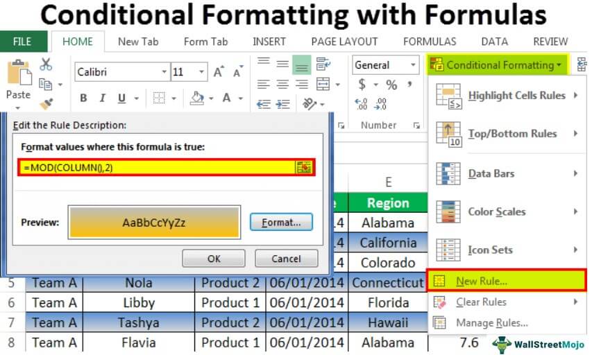
The same kind of formula can use for columns (odd and even) as well.
=INT(MOD(COLUMN(),2))
And for even columns.
=INT(MOD(COLUMN()+1,2))
5. Highlight Cells with Errors using CF
Now let’s come to another example where we will check whether a cell contains an error or not. What we need to do is just insert a formula in conditional formatting that can check the condition and return the result in TRUE or FALSE. You can even verify cells for numbers, text, or some specific values as well.

6. Create a Checklist with Conditional Formatting
Now let’s add some creativity to intelligence. You have already learned how to use a formula that is based on another cell. Here we have linked a checkbox with the B1 cell and further linked the B1 with the formula used in conditional formatting for cell A1.

Now, if you tick mark the checkbox, the value of cell B1 will turn into TRUE and cell A1 gets it conditional formatting [strikethrough].
Points to Remember
- Your formula should be a logical formula, which leads to a result as TRUE or FALSE.
- Try not to overload your data with conditional formatting.
- Always use relative and absolute references in a proper sense.
Sample File
Download this sample file from here to learn more.
More Tutorials
- AUTO FORMAT Option in Excel
- Apply Accounting Number Format in Excel
- Apply Background Color to a Cell or the Entire Sheet in Excel
- Print Excel Gridlines
- Add Page Number in Excel
- Apply Comma Style in Excel
- Apply Strikethrough in Excel
- Highlight Blank Cells in Excel
- Make Negative Numbers Red in Excel
- Cell Style (Title, Calculation, Total, Headings…) in Excel
- Change Date Format in Excel
- Highlight Alternate Rows in Excel with Color Shade
- Use Icon Sets in Excel (Conditional Formatting)
- Add Border in Excel
- Change Border Color in Excel
- Clear Formatting in Excel
- Copy Formatting in Excel
- Best Fonts for Microsoft Excel
- Hide Zero Values in Excel
⇠ Back to Advanced Excel Tutorials
The TEXT function lets you change the way a number appears by applying formatting to it with format codes. It’s useful in situations where you want to display numbers in a more readable format, or you want to combine numbers with text or symbols.
Note: The TEXT function will convert numbers to text, which may make it difficult to reference in later calculations. It’s best to keep your original value in one cell, then use the TEXT function in another cell. Then, if you need to build other formulas, always reference the original value and not the TEXT function result.
Syntax
TEXT(value, format_text)
The TEXT function syntax has the following arguments:
|
Argument Name |
Description |
|
value |
A numeric value that you want to be converted into text. |
|
format_text |
A text string that defines the formatting that you want to be applied to the supplied value. |
Overview
In its simplest form, the TEXT function says:
-
=TEXT(Value you want to format, «Format code you want to apply»)
Here are some popular examples, which you can copy directly into Excel to experiment with on your own. Notice the format codes within quotation marks.
|
Formula |
Description |
|
=TEXT(1234.567,«$#,##0.00») |
Currency with a thousands separator and 2 decimals, like $1,234.57. Note that Excel rounds the value to 2 decimal places. |
|
=TEXT(TODAY(),«MM/DD/YY») |
Today’s date in MM/DD/YY format, like 03/14/12 |
|
=TEXT(TODAY(),«DDDD») |
Today’s day of the week, like Monday |
|
=TEXT(NOW(),«H:MM AM/PM») |
Current time, like 1:29 PM |
|
=TEXT(0.285,«0.0%») |
Percentage, like 28.5% |
|
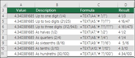
=TEXT(4.34 ,«# ?/?») |
Fraction, like 4 1/3 |
|
=TRIM(TEXT(0.34,«# ?/?»)) |
Fraction, like 1/3. Note this uses the TRIM function to remove the leading space with a decimal value. |
|
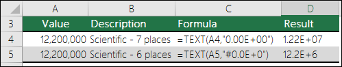
=TEXT(12200000,«0.00E+00») |
Scientific notation, like 1.22E+07 |
|
=TEXT(1234567898,«[<=9999999]###-####;(###) ###-####») |
Special (Phone number), like (123) 456-7898 |
|
=TEXT(1234,«0000000») |
Add leading zeros (0), like 0001234 |
|
=TEXT(123456,«##0° 00′ 00»») |
Custom — Latitude/Longitude |
Note: Although you can use the TEXT function to change formatting, it’s not the only way. You can change the format without a formula by pressing CTRL+1 (or  +1 on the Mac), then pick the format you want from the Format Cells > Number dialog.
Download our examples
You can download an example workbook with all of the TEXT function examples you’ll find in this article, plus some extras. You can follow along, or create your own TEXT function format codes.
Download Excel TEXT function examples
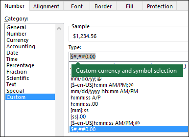
Other format codes that are available
You can use the Format Cells dialog to find the other available format codes:
-
Press Ctrl+1 (
 +1 on the Mac) to bring up the Format Cells dialog.
 -
Select the format you want from the Number tab.
-
Select the Custom option,
-
The format code you want is now shown in the Type box. In this case, select everything from the Type box except the semicolon (;) and @ symbol. In the example below, we selected and copied just mm/dd/yy.
-
Press Ctrl+C to copy the format code, then press Cancel to dismiss the Format Cells dialog.
-
Now, all you need to do is press Ctrl+V to paste the format code into your TEXT formula, like: =TEXT(B2,»mm/dd/yy«). Make sure that you paste the format code within quotes («format code»), otherwise Excel will throw an error message.

Format codes by category
Following are some examples of how you can apply different number formats to your values by using the Format Cells dialog, then use the Custom option to copy those format codes to your TEXT function.
Why does Excel delete my leading 0’s?
Excel is trained to look for numbers being entered in cells, not numbers that look like text, like part numbers or SKU’s. To retain leading zeros, format the input range as Text before you paste or enter values. Select the column, or range where you’ll be putting the values, then use CTRL+1 to bring up the Format > Cells dialog and on the Number tab select Text. Now Excel will keep your leading 0’s.
If you’ve already entered data and Excel has removed your leading 0’s, you can use the TEXT function to add them back. You can reference the top cell with the values and use =TEXT(value,»00000″), where the number of 0’s in the formula represents the total number of characters you want, then copy and paste to the rest of your range.
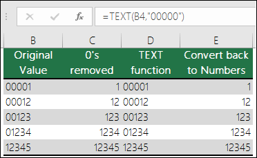
If for some reason you need to convert text values back to numbers you can multiply by 1, like =D4*1, or use the double-unary operator (—), like =—D4.
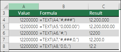
Excel separates thousands by commas if the format contains a comma (,) that is enclosed by number signs (#) or by zeros. For example, if the format string is «#,###», Excel displays the number 12200000 as 12,200,000.
A comma that follows a digit placeholder scales the number by 1,000. For example, if the format string is «#,###.0,», Excel displays the number 12200000 as 12,200.0.
Notes:
-
The thousands separator is dependent on your regional settings. In the US it’s a comma, but in other locales it might be a period (.).
-
The thousands separator is available for the number, currency and accounting formats.
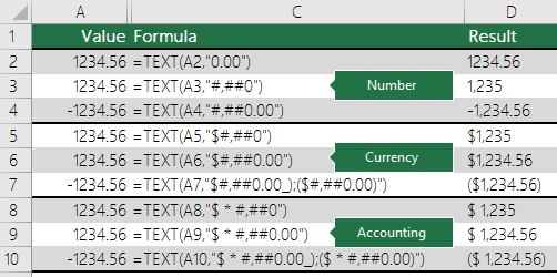
Following are examples of standard number (thousands separator and decimals only), currency and accounting formats. Currency format allows you to insert the currency symbol of your choice and aligns it next to your value, while accounting format will align the currency symbol to the left of the cell and the value to the right. Note the difference between the currency and accounting format codes below, where accounting uses an asterisk (*) to create separation between the symbol and the value.
To find the format code for a currency symbol, first press Ctrl+1 (or +1 on the Mac), select the format you want, then choose a symbol from the Symbol drop-down:
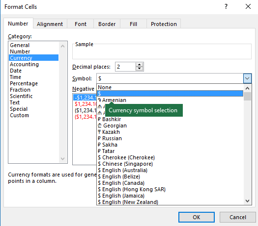
Then click Custom on the left from the Category section, and copy the format code, including the currency symbol.
Note: The TEXT function does not support color formatting, so if you copy a number format code from the Format Cells dialog that includes a color, like this: $#,##0.00_);[Red]($#,##0.00), the TEXT function will accept the format code, but it won’t display the color.
You can alter the way a date displays by using a mix of «M» for month, «D» for days, and «Y» for years.
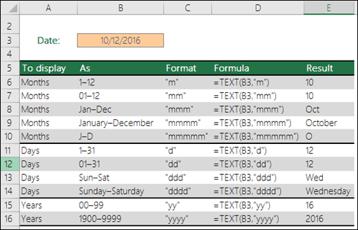
Format codes in the TEXT function aren’t case sensitive, so you can use either «M» or «m», «D» or «d», «Y» or «y».
You can alter the way time displays by using a mix of «H» for hours, «M» for minutes, or «S» for seconds, and «AM/PM» for a 12-hour clock.
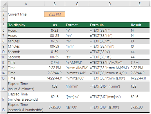
If you leave out the «AM/PM» or «A/P», then time will display based on a 24-hour clock.
Format codes in the TEXT function aren’t case sensitive, so you can use either «H» or «h», «M» or «m», «S» or «s», «AM/PM» or «am/pm».
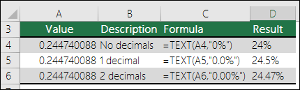
You can alter the way decimal values display with percentage (%) formats.
You can alter the way decimal values display with fraction (?/?) formats.
Scientific notation is a way of displaying numbers in terms of a decimal between 1 and 10, multiplied by a power of 10. It is often used to shorten the way that large numbers display.
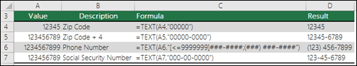
Excel provides 4 special formats:
-
Zip Code — «00000»
-
Zip Code + 4 — «00000-0000»
-
Phone Number — «[<=9999999]###-####;(###) ###-####»
-
Social Security Number — «000-00-0000»
Special formats will be different depending on locale, but if there aren’t any special formats for your locale, or if these don’t meet your needs then you can create your own through the Format Cells > Custom dialog.
Common scenario
The TEXT function is rarely used by itself, and is most often used in conjunction with something else. Let’s say you want to combine text and a number value, like “Report Printed on: 03/14/12”, or “Weekly Revenue: $66,348.72”. You could type that into Excel manually, but that defeats the purpose of having Excel do it for you. Unfortunately, when you combine text and formatted numbers, like dates, times, currency, etc., Excel doesn’t know how you want to display them, so it drops the number formatting. This is where the TEXT function is invaluable, because it allows you to force Excel to format the values the way you want by using a format code, like «MM/DD/YY» for date format.
In the following example, you’ll see what happens if you try to join text and a number without using the TEXT function. In this case, we’re using the ampersand (&) to concatenate a text string, a space (» «), and a value with =A2&» «&B2.
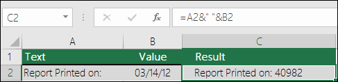
As you can see, Excel removed the formatting from the date in cell B2. In the next example, you’ll see how the TEXT function lets you apply the format you want.
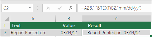
Our updated formula is:
-
Cell C2:=A2&» «&TEXT(B2,»mm/dd/yy») — Date format
Frequently Asked Questions
Yes, you can use the UPPER, LOWER and PROPER functions. For example, =UPPER(«hello») would return «HELLO».
Yes, but it takes a few steps. First, select the cell or cells where you want this to happen and use Ctrl+1 to bring up the Format > Cells dialog, then Alignment > Text control > check the Wrap Text option. Next, adjust your completed TEXT function to include the ASCII function CHAR(10) where you want the line break. You might need to adjust your column width depending on how the final result aligns.
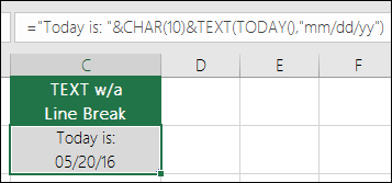
In this case, we used: =»Today is: «&CHAR(10)&TEXT(TODAY(),»mm/dd/yy»)
This is called Scientific Notation, and Excel will automatically convert numbers longer than 12 digits if a cell(s) is formatted as General, and 15 digits if a cell(s) is formatted as a Number. If you need to enter long numeric strings, but don’t want them converted, then format the cells in question as Text before you input or paste your values into Excel.
See Also
Create or delete a custom number format
Convert numbers stored as text to numbers
All Excel functions (by category)
Excel, by default, has already provided us with many types of conditional formatting to perform with our data. Still, we want to do the formatting on specific criteria or formulas as a user. We can do that by choosing the “Home” tab of the “Conditional Formatting” section. Then, when we click on the “New Rule,” we can find an option for conditional formatting with formulas where we can insert formulas that will define the cells to format.
The conditional formatting with formula is changing the format of the cells based on the condition or criteria given by the user. For example, you might have used conditional formattingConditional formatting is a technique in Excel that allows us to format cells in a worksheet based on certain conditions. It can be found in the styles section of the Home tab.read more to highlight the top value in the range and duplicate values.
A good thing is we have formulas in conditional formatting in excel. All the formulas should be logical. The result will be either “TRUE” or “FALSE”. If the logical test passes, we will get conditional formatting. If the excel logical testA logical test in Excel results in an analytical output, either true or false. The equals to operator, “=,” is the most commonly used logical test.read more fails, we will get nothing.
Table of contents
- Conditional Formatting with Formulas in Excel
- Overview
- How to Use Excel Conditional Formatting with Formulas?
- #1 – Highlight Cells which has Values Less than 500
- #2 – Highlight One Cells Based on Another Cell
- #3 – Highlight All the Empty Cells in the Range
- #4 – Use AND Function to Highlight Cells
- #5- Use OR Function to Highlight Cells
- #6 – Use COUNTIF Function to Highlight Cells
- #7 – Highlight Every Alternative Row
- #8 – Highlight Every Alternative Column
- Things to Remember
- Recommended Articles
Overview
Let me introduce you to conditional formatting with the formula window.
In the below section of the article, we will see a wide variety of examples for applying conditional formatting with formulas.
How to Use Excel Conditional Formatting with Formulas?
You can download this Excel Conditional Formatting with Formulas Template here – Excel Conditional Formatting with Formulas Template
#1 – Highlight Cells which has Values Less than 500
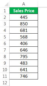
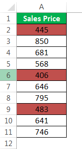
Assume you are working with the sales numbers given below.
- Below is the sales price per unit.

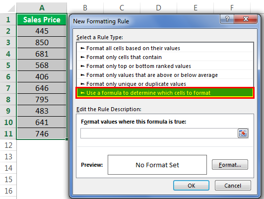
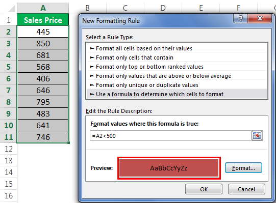
- Then, we must go to Conditional Formatting and click on New Rule.

- Now, select Use a formula to determine which cells to format.

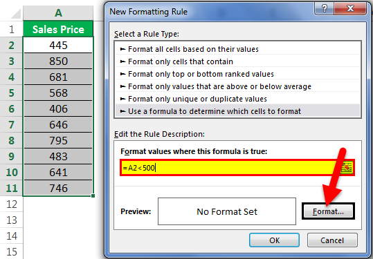
- Now, under Format values where a formula is true, apply the formula as c500 and click on Format to use the excel formatting.

- Then, we must select the format as per our choice.

- Now, we can see the preview of the format in the preview box.

- Now, click on OK to complete the formatting. As a result, it has highlighted all the cells with a number c500.

#2 – Highlight One Cells Based on Another Cell
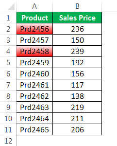
We can highlight one cell based on another cell’s value. For example, assume we have “Product” and “Sales Price” data in the first two columns.
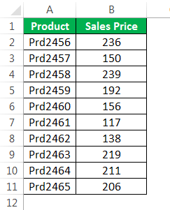
We need to highlight the products from the above table if the sale price is >220.
- Step 1: First, we must select the “Product” range, go to “Conditional Formatting,” and click on “New Rule.”
- Step 2: In the formula, we must apply the formula as B2 > 220.
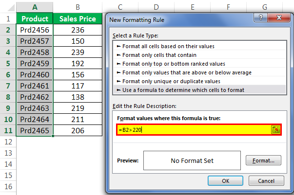
- Step 3: Then, click on the “Format” key and apply the format as per choice.

- Step 4: Then click “OK.” Now, we can see that formatting is ready.
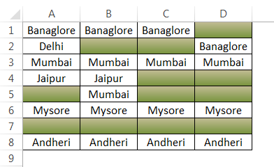
#3 – Highlight All the Empty Cells in the Range
Assume we have the below-given data.
We must highlight all the blank or empty cells in the above data because we need to use the ISBLANK formulaISBLANK in Excel is a logical function that checks if a target cell is blank or not. It returns the output “true” if the cell is empty (blank) or “false” if the cell is not empty. It is also known as referencing worksheet function and is grouped under the information function of Excel
read more in the Excel conditional formatting.
Apply the below formula in the formulas section.

Now, first, we must select the formatting as per our wish.
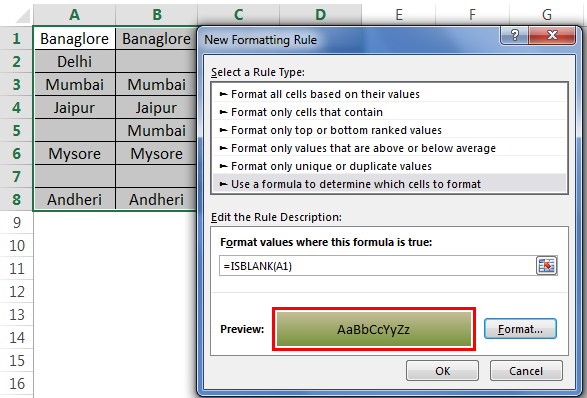
Click on “OK.” It will highlight all the empty cells in the selected range.
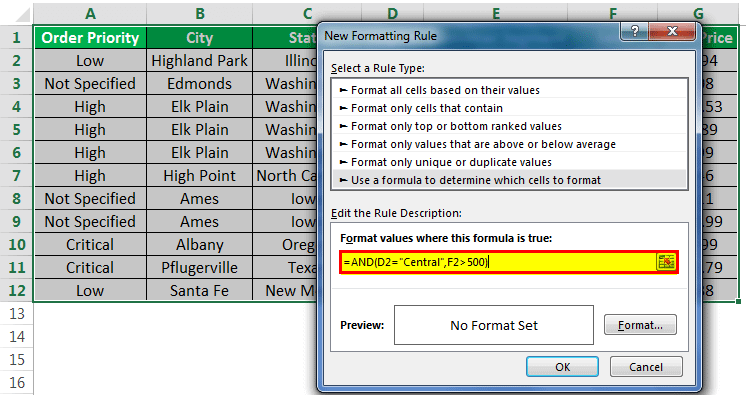
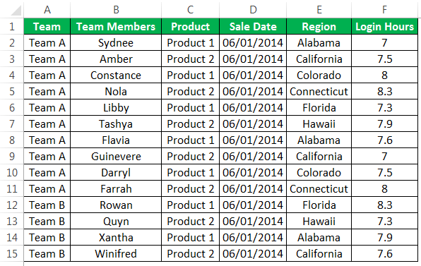
#4 – Use AND Function to Highlight Cells
Consider the below data for this formula.
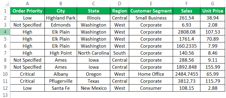
If the region is Central and the sales value is >500, we need to highlight the complete row.
- Step 1: We must select the entire data first.
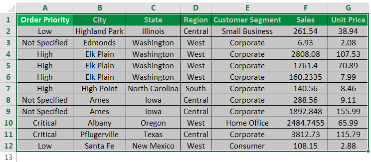
- Step 2: Next, we need to use the AND excel functionThe AND function in Excel is classified as a logical function; it returns TRUE if the specified conditions are met, otherwise it returns FALSE.read more to test two conditions here. Both the conditions should be “TRUE.” Then, we must apply the below formula.
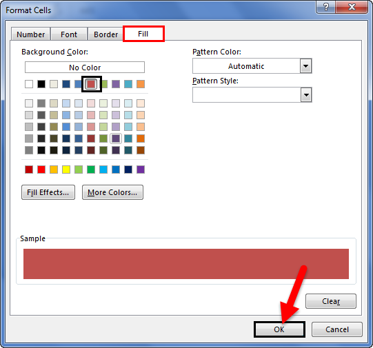
- Step 3: Then, click on “Format.”
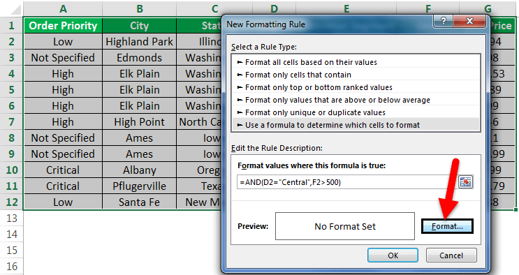
- Step 4: We must go to “FILL” and select the required color and effects.

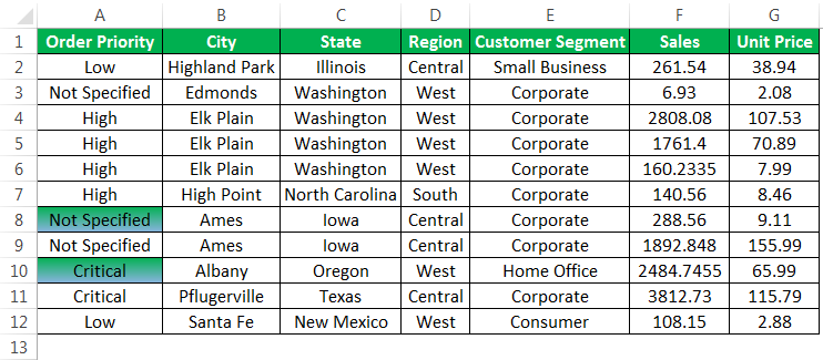
- Step 5: Now, click on “OK.” As a result, we can see the rows highlighted if both the conditions are “TRUE.”
#5- Use OR Function to Highlight Cells
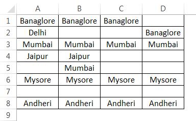
For example, consider the below data.
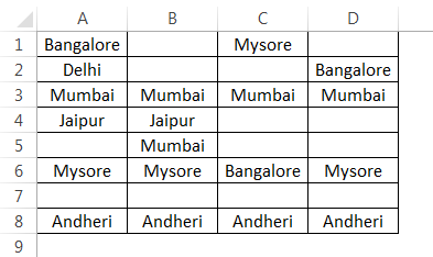
We want to highlight the city names “Bangalore” and “Mysore” in the above data range.
- Step 1: We must select the data first, go to “Conditional Formatting,” and click on “New Rule.”
- Step 2: Since we need to highlight either of the two value cells, we must apply the OR excel functionThe OR function in Excel is used to test various conditions, allowing you to compare two values or statements in Excel. If at least one of the arguments or conditions evaluates to TRUE, it will return TRUE. Similarly, if all of the arguments or conditions are FALSE, it will return FASLE.read more.
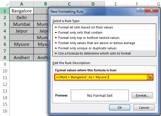
- Step 3: Then, click on the “Format” and select the required format.
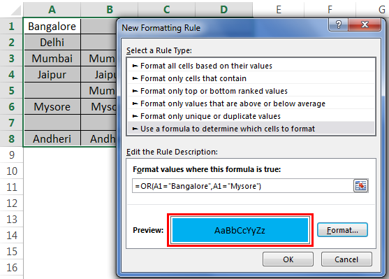
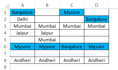
- Step 4: Once the formatting is applied, click on “OK” to complete the task. As a result, a formula would highlight all the cells with values “Bangalore” and “Mysore.”
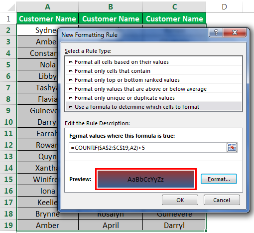
#6 – Use COUNTIF Function to Highlight Cells
Assume you are working with the customer database. First, you need to identify all the clients whose names appear more than five times on the list. Below is the data.
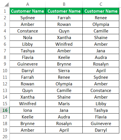
First, we must select the data and apply the COUNTIF formula in the formula section.

Then, click on the “Format” and apply the required formatting.
Consequently, the formula will highlight all the names if the count is more than 5.
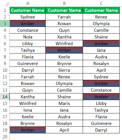
Amber is the only name that appears more than five times on the list.
#7 – Highlight Every Alternative Row
We can also have the formula to highlight every alternative row in excelIn Excel, we can highlight every other row in one of three ways: using an Excel table, conditional formatting, or custom formatting.read more of the data. For example, assume below is the data we are working on.
We will select the data first and apply the below formula.
=MOD(ROW (), 2)
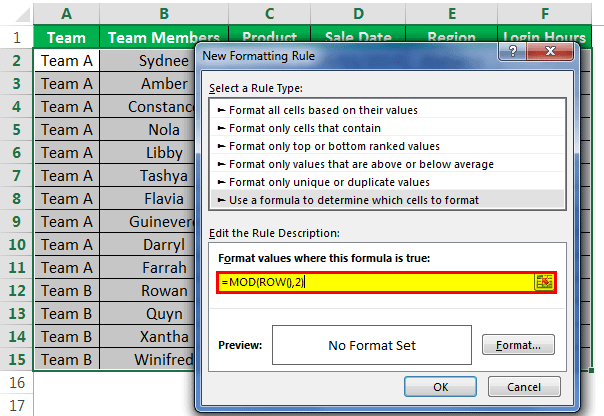
We will apply the format as per our wish and click on “OK.” As a result, we have every alternate row highlighted by the formula.

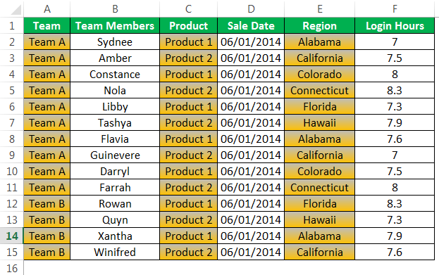
#8 – Highlight Every Alternative Column
Like how we have highlighted every alternative row similarly, we can highlight every alternate column. Again, consider the same data for the example.
And apply the below formula:
=MOD(COLUMN(), 2)
Now, copy the above formula and apply it in the formula section of the conditional formatting.
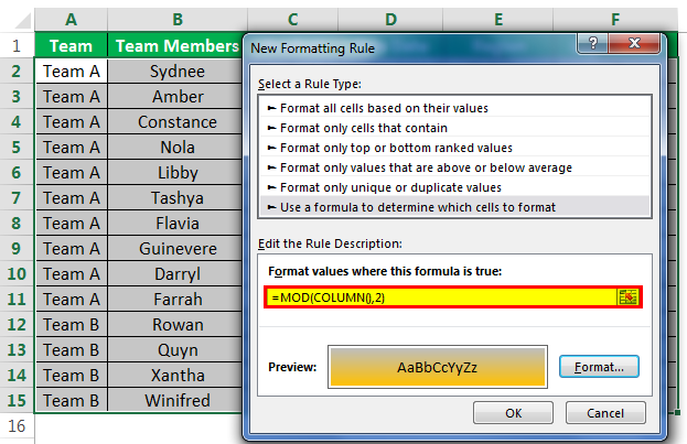
Click on “OK.” We can see now that it has highlighted the alternative row as shown below.
If we wish to leave out the first column and highlight the second column, we can use the below formula.
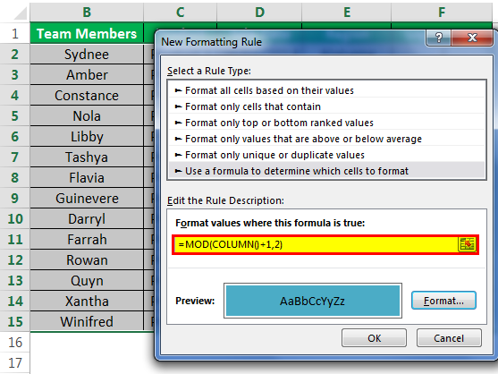
Therefore, this formula will highlight the alternative column starting from the second column.
Things to Remember
- Conditional formatting accepts only logical formulas whose results are only either “TRUE” or “FALSE.”
- A preview of conditional formatting is just an indication of how formatting looks.
- We must never use absolute reference as in the formula. When applying the formula, if we select the cell directly, it would make it an absolute reference. We need to make it to a relative reference in excelIn Excel, relative references are a type of cell reference that changes when the same formula is copied to different cells or worksheets. Let’s say we have =B1+C1 in cell A1, and we copy this formula to cell B2 and it becomes C2+D2.read more.
Recommended Articles
This article has been a guide to Excel Conditional Formatting with Formulas. We discuss using conditional formatting using formulas like COUNTIF, AND, OR, MOD, etc., practical examples, and a downloadable Excel template. You may learn more about Excel from the following articles: –
- How to Use Conditional Formatting for Dates?
- How to Create Excel KPI Dashboard?
- Conditional Formatting in Excel VBA
- VBA COUNTIF
Условное форматирование с использованием формул
В Excel условное форматирование позволяет использовать формулы в критериях вместо значений. В таком случаи критерий автоматически получает результирующие значение, которое выдает формула в результате вычислений.
Условное форматирование по формуле
Формулы в качестве критериев можно использовать практически любые, которые возвращают значения. Но для логических формул (возвращающие значения ИСТИННА или ЛОЖЬ) в Excel предусмотрен отдельный тип правил.
При использовании логических формул в качестве критериев следует:
- Выбрать инструмент: «Главная»-«Стили»-«Условное форматирование»-«Управление правилами».
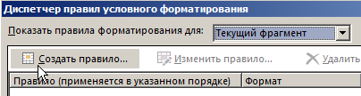
- В появившемся окне «Диспетчер правил условного форматирования» нажать на кнопку «Создать правило».
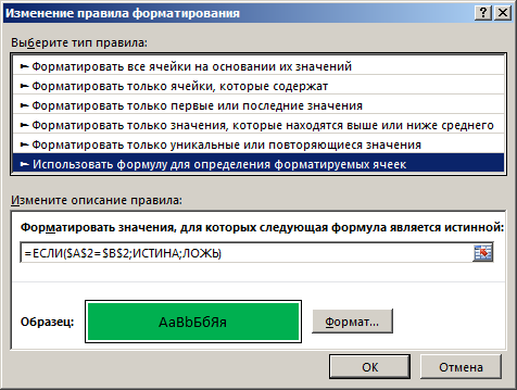
- В списке опций «Выберите тип правила:» выберите опцию «Использовать формулу для определения форматируемых ячеек».
- В поле ввода «Форматировать значения, для которых следующая формула является истинной» ввести логическую формула, а нажав на кнопку «Формат» указать стиль оформления ячеек.

Правила использования формул в условном форматировании
При использовании формул в качестве критериев для правил условного форматирования следует учитывать некоторые ограничения:
- Нельзя ссылаться на данные в других листах или книгах. Но можно ссылаться на имена диапазонов (так же в других листах и книгах), что позволяет обойти данное ограничение.
- Существенное значение имеет тип ссылок в аргументах формул. Следует использовать абсолютные ссылки (например, =СУММ($A$1:$A$5) на ячейки вне диапазона условного форматирования. А если нужно ссылаться на несколько ячеек непосредственно внутри диапазона, тогда следует использовать смешанные типы ссылок (например, A$1).
- Если в критериях формула возвращает дату или время, то ее результат вычисления будет восприниматься как число. Ведь даты это те же целые числа (например, 01.01.1900 – это число 1 и т.д.). А время это дробные значения части от целых суток (например, 23:15 – это число 0,96875).
Иногда встроенные условия формата ячеек не удовлетворяют всех потребностей пользователей. Добавление собственной формулы в условное форматирование обеспечивает дополнительную функциональность, которая не доступна в строенных функциях данного инструмента. Excel предоставляет возможность использовать много критериев или применять сложные вычисления, что дает широкое поле к применению сложных настроек критериев для автоматически генерированного презентабельного экспонирования важной информации.
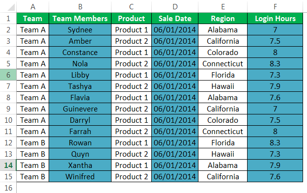
Практический пример использования логических функций и формул в условном форматировании для сравнения двух таблиц на совпадение значений.
When working with formulas, there is always a possibility that someone (or even you) may delete a cell (or clear the contents of a cell/range) that has formulas in it.
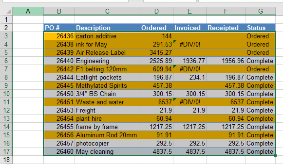
Wouldn’t it be better if these cells with formulas are highlighted or formatted in a way that makes these stand out? This would help ensure you don’t end up deleting these cells by mistake.
In this tutorial, I will show you how to auto-format formulas in Excel (i.e., highlight the cells with formulas).
So let’s get started!
Autoformat Formulas using Conditional Formatting
The easiest way to autoformat cells with formulas is to use conditional formatting.
If you can somehow identify cells that have formulas, you can easily format these differently using conditional formatting.
And this is where you can use the ISFORMULA function, a function that was introduced in Excel 2013.
The ISFORMULA function checks whether a cell has a formula in it or not, and if it has a formula, then it returns TRUE (else FALSE).
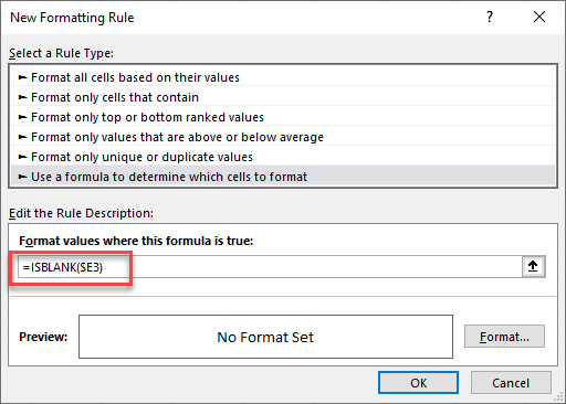
Below are the steps to use this function in Conditional Formatting to autoformat formulas in Excel:
- Select the dataset in which you want to format the cells with formulas
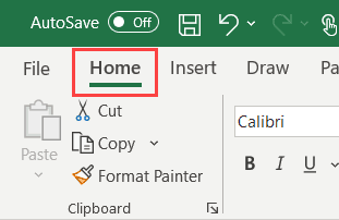
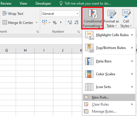
- Click the Home tab

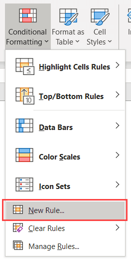
- In the Styles group, click on Conditional Formatting

- Click on New Rule

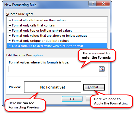
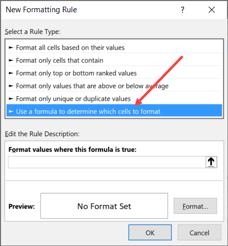
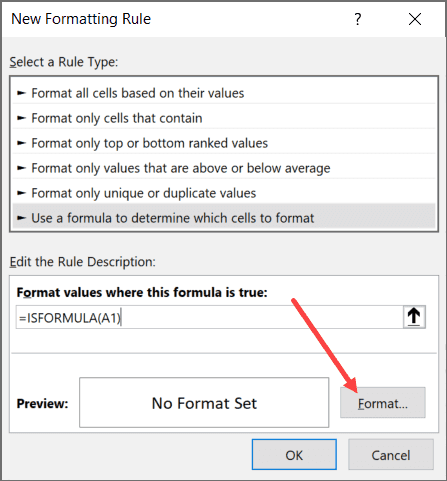
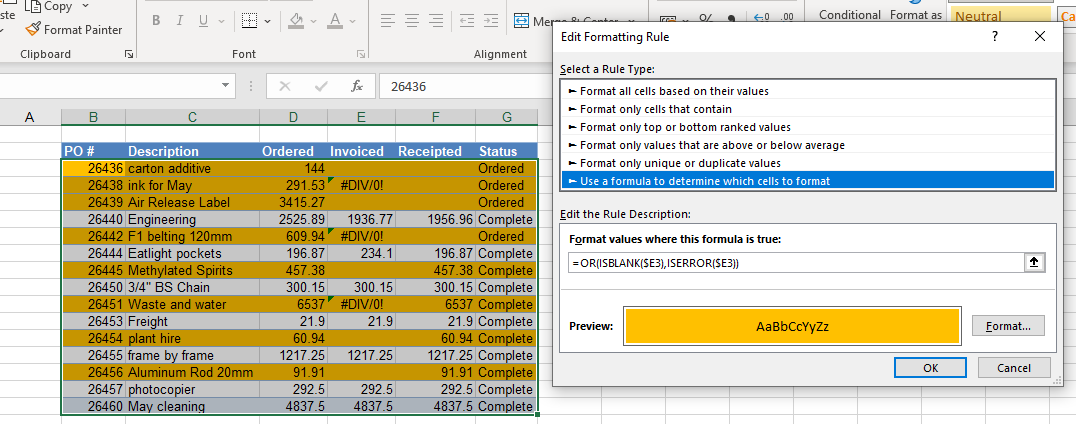
- In the New Formatting Rule dialog box that opens, select ‘Use a formula to determine which cells to format’

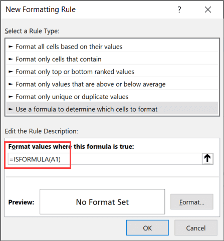
- In the formula field, enter the formula =ISFORMULA(A1)
- Click on the Format button
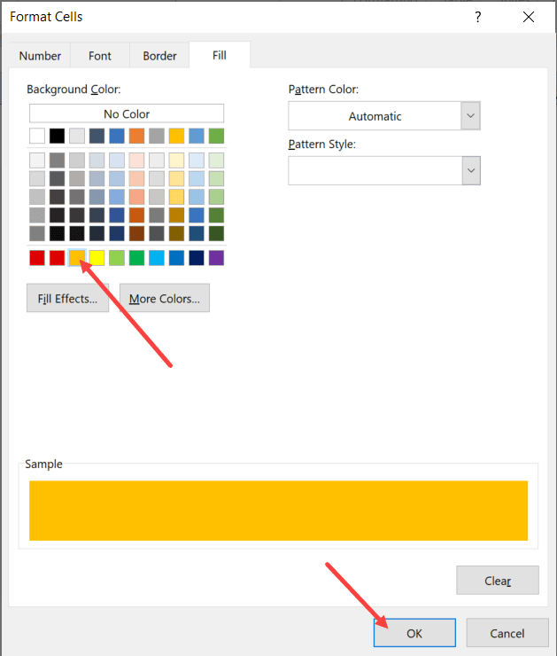
- In the Format Cells dialog box that opens, specify the formatting that you want to apply to the cells with formulas. In my case, I am using the orange cell fill color

- Click OK
The above steps would instantly autoformat all the cells that have a formula in it.
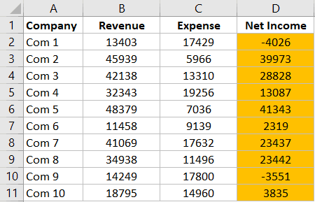
Not only this, in case you change any of the cells and add a formula to it, the color would automatically change. Since conditional formatting is dynamic and checks for each cell every time there is a change in the worksheet, the above steps make sure cells are automatically highlighted.
While this is my preferred method to autoformat formulas in Excel, there is another way as well.
Also read: How to Strikethrough in Excel (5 Ways + Shortcuts)
Autoformat Formulas using Go To Special
Unlike the Conditional formatting method, this one is not dynamic.
So when you do this once, it will select all the cells with formulas and you can format them at one go. But if now you change any cell and add a formula, that cell will not get highlighted.
Below are the steps to use Go To Special to select all cells with Formulas and then format these:
- Select the dataset in which you want to format the cells with formulas
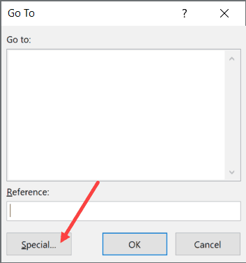
- Hit the F5 key – this will open the Go To dialog box
- Click on the Special button

- In the Go To Special dialog box, Click on Formulas

- Click OK
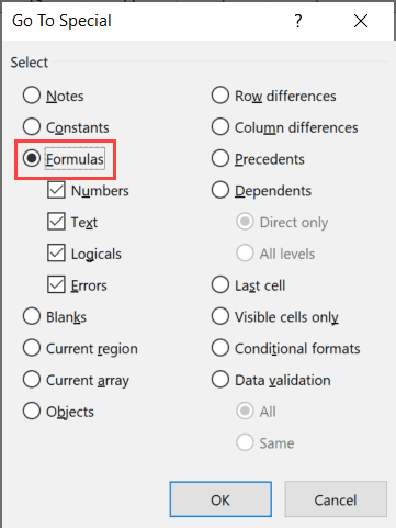
The above steps would select all the cells that have formulas in it. Once these cells are selected, you can apply whatever formatting you want. For example, you can apply a cell color or can change the font to bold.
As I mentioned, now if you add a new formula to the range, it will not get autoformatted. You will have to repeat the same process again.
Format Formulas using VBA
Another quick method to quickly format cells with formulas is by using VBA.
This method does exactly the same thing as the one the previous one (using Go To Special), but with a single line of code.
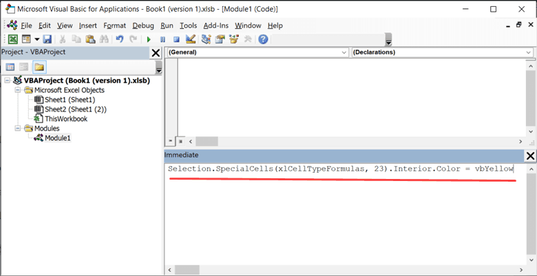
Below is the VBA code that will instantly highlight all the cells that have formulas in it in yellow color:
Selection.SpecialCells(xlCellTypeFormulas, 23).Interior.Color = vbYellow
This code first selects all the cells that have formulas and then applies the yellow color (specified by vbYellow).
Here are the steps to use this VBA macro code:
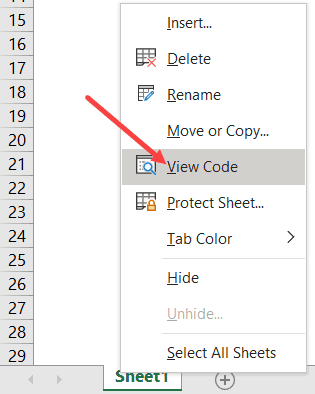
- Right-click on the active sheet tab name (the one where you have the data with formulas that you want to format).
- Click on View Code

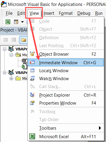
- If you don’t see the ‘Immediate window’ in the VB Editor already, click on the ‘View’ option in the menu and then click on ‘Immediate Window’

- Copy and paste the above VBA code in the ‘Immediate Window’

- Place the cursor at the end of the line
- Hit the Enter key
The above code first identifies all the cells with formulas and then applies the yellow color. You can modify the code in case you want to apply some other type of formatting.
So these are two simple ways to quickly autoformat formulas in Excel.
Hope you found this tutorial useful!
You may also like the following Excel tutorials:
- How to Format Phone Numbers in Excel
- How to Clear Contents in Excel without Deleting Formulas
- How to Delete a Comment in Excel (or Delete ALL Comments)
- Excel Showing Formula Instead of Result
- SUMPRODUCT vs SUMIFS Function in Excel
- How to Convert Decimal to Fraction in Excel
- How to Shade Every Other Row in Excel
- How to Autofill Dates in Excel (Autofill Months/Years)
- How to Apply Comma Style in Excel
- How to Increase/Decrease Indent in Excel? (Easy Shortcut)
This tutorial demonstrates how to apply conditional formatting based on a formula in Excel and Google Sheets.
Conditional Formatting in Excel comes with plenty of preset rules to enable you to quickly format cells according to their content. These preset rules do, however, have limitations, which is where using a formula to determine the format of a cell comes into play. This gives you much greater flexibility over your conditional formatting.
Conditional Formatting Formula Rules
Equal To
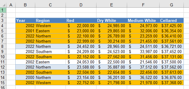
- Highlight the cells where you want to set the conditional formatting and then, in the Ribbon, select Home > Conditional Formatting > New Rule.
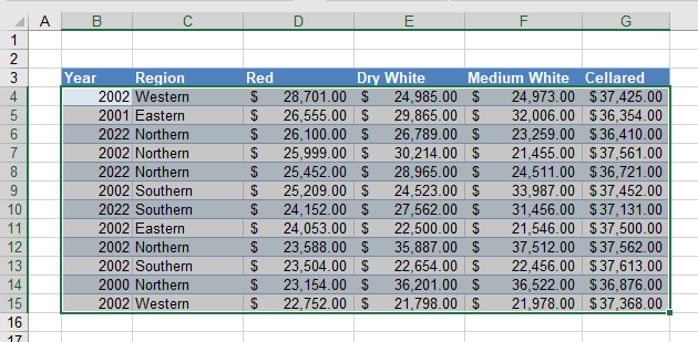
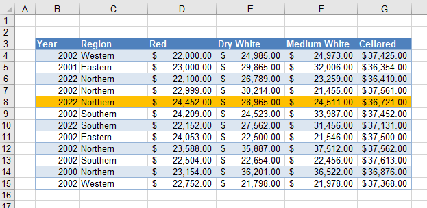
- Select Use a formula to determine which cells to format, and enter the formula:
=$C4=”Western”
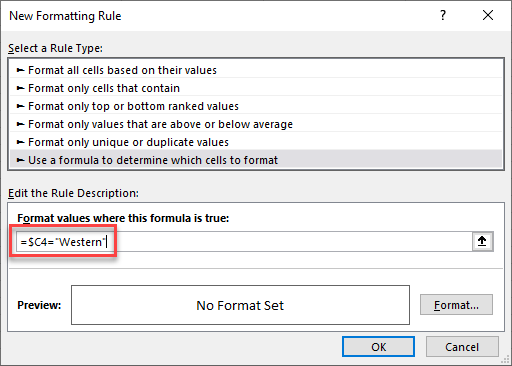
You always need to start your formula with an equal sign.
The formula tests whether the result is TRUE or FALSE much like the traditional Excel IF statement, but in the case of conditional formatting, you do not need to add the true and false conditions. If the formula returns TRUE, then formatting you set in the Format part of the rule is applied to the relevant cells.
You need to use a mixed reference in this formula ($C4) in order to lock the column (make it absolute) but make the row relative. This enables the formatting to format the entire row instead of just a single cell that meets the criteria.
When the rule is evaluated for all the cells in the range, the row changes, but the column does not. This causes the rule to ignore the values in any of the other columns and just concentrate on the values in Column C. If Column C of that row contains the word Western, the formula result is TRUE, and the formatting is applied for the whole row.
- Click Format… and select your desired formatting.
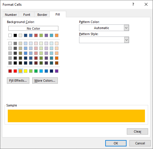
- Click OK and then OK again to view the result.
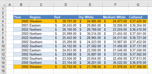
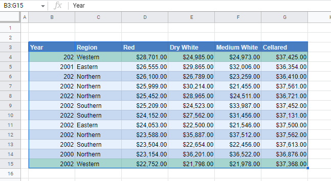
The rows where Column C is Western are highlighted, while other rows are not. In the example above, just two rows end up highlighted.
Not Equal
If you want to create an opposite rule, you can use the <> (not equal to) operator instead of =.
=$C4<>”Western”
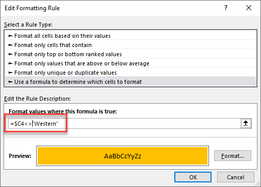
This results in the opposite: Most of the rows are now highlighted!
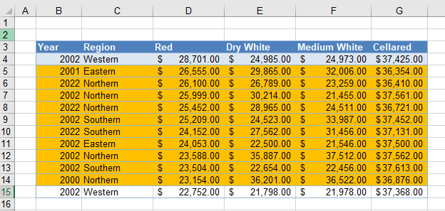
Greater Than
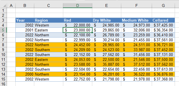
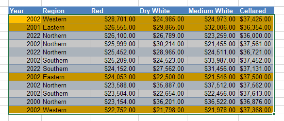
You can also test for greater than using a formula. For example, you can use a formula to check if the values in Column D are greater than $23,000.
=$D4>23000
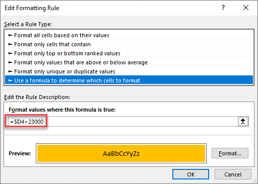
This rule highlights only rows where the value in Column D is greater than $23,000.
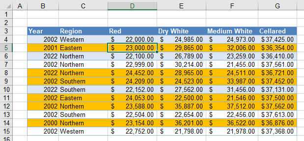
Greater Than or Equal To
Similarly, you could highlight the rows where the value in Column D is greater than or equal to $23,000 with this formula below:
=$D4>=23000

The result for this formula would be slightly different: Rows where the Red value is exactly $23,000 are also highlighted (here, Row 5).
Less Than
Swapping the > sign for a < sign tests for values that are less than $23,000.
=$D4<23000

Now only rows where Red is less than $23,000 are highlighted.
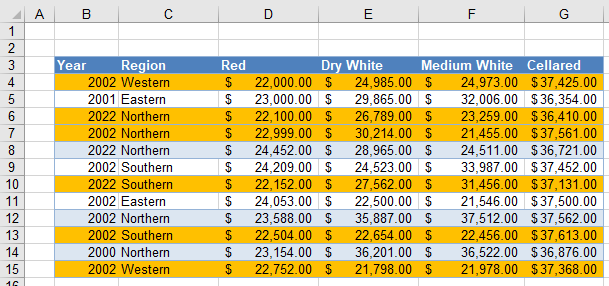
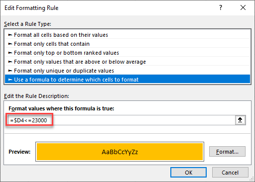
Less Than or Equal To
To change the test to include the target value (e.g., $23,000), use <=.
=$D4<=23000
Now, any rows in which Column D is equal to $23,000 are also highlighted.
Create Rules With OR, AND
OR Formula
You can create a more complicated rule by incorporating the Excel OR Function to expand the formula to look for two or more values.
- Enter the formula:
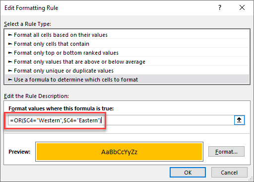
=OR($C4=”Western”,$C4=”Eastern”)
- Click on the Format… button and select your desired formatting, and then click OK to return to Excel.
This highlights all rows where the Region is Western or Eastern.
AND Formula
Similarly, you can create a rule using AND. This would mean checking the values in two or more columns.
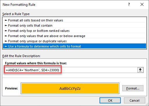
The formula above checks whether the text in Column C is Northern and the value in the corresponding row in Column D is greater than $23,000.
This conditional formatting rule highlights only the rows where both conditions are met.
IF Formula
You do not necessarily have to add an IF statement to the formula when you are creating it in a conditional formatting rule as the conditional formatting is always going to apply the rule if the formula that you have created returns a true value.
So, for example, this formula:
=IF($C4=”Western”,TRUE,FALSE)
and this formula
$C4=”Western”
both apply the same conditional formatting to your worksheet.
Built-in Excel Functions
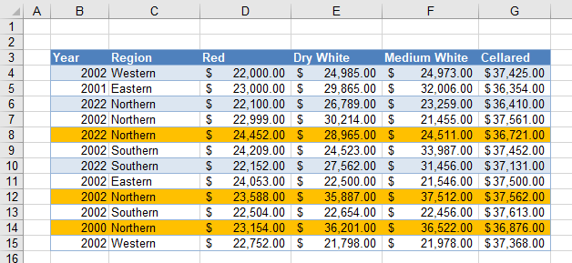
Many built-in Excel functions can be used in conditional formatting such as ISBLANK, ISERROR, ISEVEN, ISNUMBER, etc.
ISBLANK Function
You can use the ISBLANK Function to create a rule to find rows that contain blank or empty cells in the worksheet.
- Highlight the range and then, in the Ribbon, select Home > Conditional Formatting > New Rule.
- Type in the formula:
=ISBLANK($E3)
- Click on the Format… button and select your desired formatting and then click OK to return to Excel.
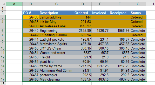
ISBLANK With OR
You can expand this to include blank cells or cells with an error in them.
- Type in the formula
=OR(ISBLANK($E3),ISERROR($E3))
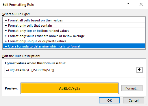
- Click on the Format… button and select your desired formatting and then click OK to return to Excel.
Other Functions in Conditional Formatting
There are a variety of other functions that can be used in creating conditional formatting formula-based rules.
- COUNTIFS – counts cells that meet a certain condition (useful for highlighting duplicates)
- LARGE – finds the kth largest value
- MAX – finds the largest number
- MIN – finds the smallest number
- MOD – returns the remainder after division (useful for highlighting every other row)
- NOT – changes TRUE to FALSE and vice versa
- NOW – returns the current date and time (useful for conditionally formatting dates and times)
- ROW – returns the number of rows in an array
- SEARCH – searches for a string of text within another string (useful for finding specific text)
- TODAY – returns the current date (useful for applying conditional formatting to dates)
- VLOOKUP – returns the result of a vertical lookup
- WEEKDAY – returns the day of the week
- XLOOKUP – a new, more powerful lookup function
For example, you can use the MAX Function to highlight the row that contains the maximum value in a specified column.
=$D4=MAX($D:$D)
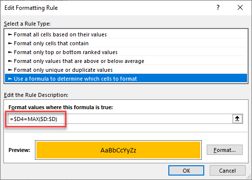
Now, only the row with the maximum value in Column D is highlighted.
If you are struggling to get a formula to work when creating a conditional formatting rule, it is a good idea to test the formula first in your Excel sheet. Once you have it right there, you can incorporate it in your rule.
Conditional Formatting Based on Formula in Google Sheets
Conditional Formatting works much the same in Google Sheets as it does in Excel.
- Highlight the cells where you want to set the conditional formatting and then, in the Menu, select Format > Conditional formatting.
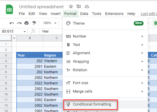
- Make sure the Apply to range is correct, and then select Custom formula is from the Format rules drop-down box. Type in the formula.
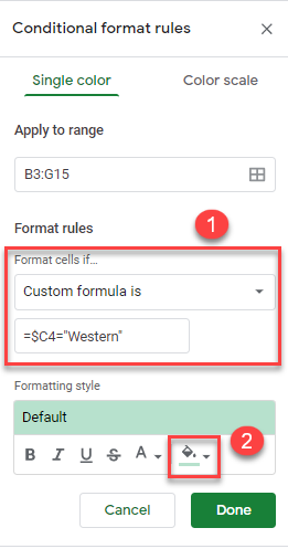
- Then, select your formatting style and click Done.
You can also use greater than, greater than or equal to, less than, and less than or equal to in Google Sheets.
AND and OR also work, as well the other functions listed above for Excel (except for XLOOKUP, which does not exist in Google Sheets).
In this article, we will learn How to perform Conditional Formatting with formula in Excel.
Why do we use conditional formatting to highlight cells in Excel ?
Conditional Formatting is used to highlight the data on the basis of some criteria. It would be difficult to see various trends just for examining your Excel worksheet. Conditional Formatting provides a way to visualize data and make worksheets easier to understand. It allows you to apply the formatting basis on the cell values such as colours, icons and data bars.
Excel Conditional formatting gives you inbuilt formulation like Highlight cells rules or top/bottom rules. These will help you achieve formulation using simple steps.
Choose the New rule to create a customized formula for highlighting cells. For example Highlight sales values where sales values are in between 150 to 1000. For this we use Conditional formatting. Try the formula in adjacent cells before applying in the conditional formatting formula box.
Formula box in Conditional formatting
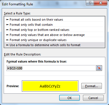
After selecting the New rule in conditional formatting. Select the Use a formula to determine which cells to format -> it will open the formula box as shown in the image above. Use the formula in it and select the type of formatting to choose using Format option (like Yellow background as shown in the image).
How to solve the problem?
For this we will be using the Conditional formatting obviously. And we can use any of the two functions SEARCH function or FIND function. The difference is SEARCH function, is case insensitive which means it will match any of substrings «ABC», «Abc», «aBc», «ABc», if matched with «abc». FIND function is case sensitive which matches only substring «abc», if matched with «abc». Below shown is the generic formula to solve this problem.
SEARCH Formula Syntax:
FIND Formula Syntax:
sp_val : specific or particular value to match with.
cell : cell to check
Example :
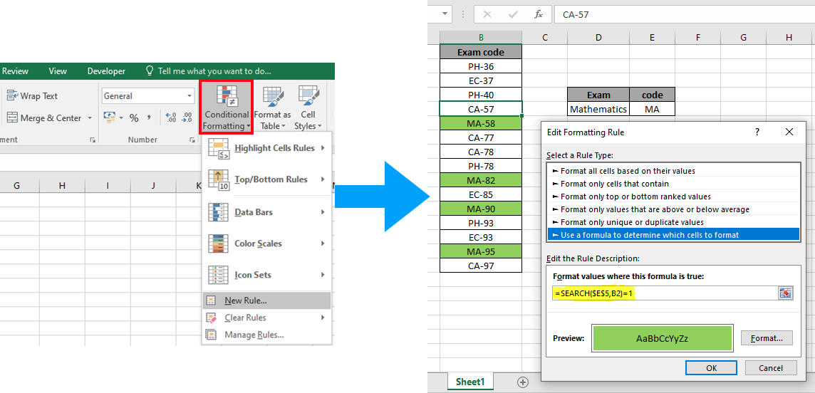
All of these might be confusing to understand. Let’s understand it better via running the formula on some values. Here we have some university exam codes. We need to highlight the mathematics exam codes. Mathematics Exam code begins with «MA».
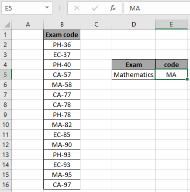
What we need here is to check each cell which starts with «MA».
Go to Home -> Conditional formatting -> New Rule
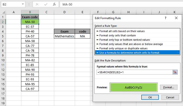
A dialog box appears in front select Use a formula to determine which cells to format -> input the below formula under the Format values where this formula is True:
Use the formula:
Explanation:
- Search matches the string in the cell value.
- Search function returns the position of occurrence of the substring in text.
- If the position matches with 1 i.e. the start of the cell. The formula returns True if matched or else False.
- True value in conditional formatting formats the cell as required.
- Customize the cell format by clicking the Format button in the right bottom of the dialog box as shown below.
- The format will will displayed adjacent to the Format button.
The background color gets Green ( highlight formatting) as you click Ok as shown above. Now copy the formula to the rest of cells using the Ctrl + D or dragging down form right bottom of B2 cell.
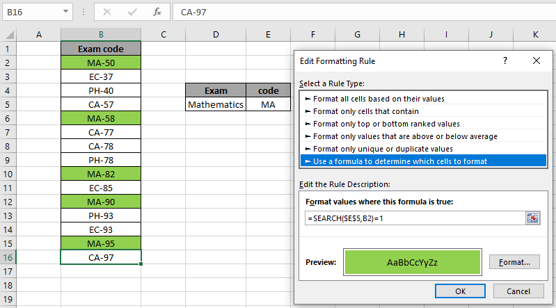
As you can see all the mathematics exam codes are highlighted. You can input specific value substring, with quotes(«) in the formula along with an example solved using the FIND function as shown below.
FIND function is case sensitive function :
FIND function returns the position of the occurrence of the find_text value in the cell value. The difference occurs if the value you are trying to match must be case sensitive. See the below formula and snapshot to understand How to highlight cells that begin with specific value in Excel.
Use the formula :
B2 : within_text
«MA» : find_text substring
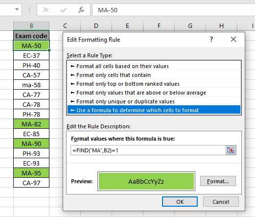
As you can see the lowercase exam code «ma-58» doesn’t match the substring «MA» as we used the FIND function here. So, it’s preferable to use the SEARCH function with conditional formatting. Conditional Formatting provides a way to visualize data and make worksheets easier to understand. You can perform various tasks using the different features of conditional formatting in Excel.
Here are all the observational notes regarding using the formula.
Notes:
- Conditional formatting allows you to apply the formatting basis on the cell values such as colours, icons and data bars.
- The formula works for text and numbers both.
- SEARCH function is case insensitive function.
Hope you understood How to perform Conditional Formatting with formula in Excel. Explore more articles on Excel matching and highlighting cells with formulas here. If you liked our blogs, share it with your friends on Facebook. And also you can follow us on Twitter and Facebook. We would love to hear from you, do let us know how we can improve, complement or innovate our work and make it better for you. Write to us at info@exceltip.com.
Related Articles:
Find the partial match number from data in Excel : find the substring matching cell values using the formula in Excel
How to Highlight cells that contain specific text in Excel : Highlight cells based on the formula to find the specific text value within the cell in Excel.
Conditional formatting based on another cell value in Excel : format cells in Excel based on the condition of another cell using some criteria.
IF function and Conditional formatting in Excel : How to use IF condition in conditional formatting with formula in excel.
Perform Conditional Formatting with formula 2016 : Learn all default features of Conditional formatting in Excel
Conditional Formatting using VBA in Microsoft Excel : Highlight cells in the VBA based on the code in Excel.
Popular Articles :
How to use the IF Function in Excel : The IF statement in Excel checks the condition and returns a specific value if the condition is TRUE or returns another specific value if FALSE.
How to use the VLOOKUP Function in Excel : This is one of the most used and popular functions of excel that is used to lookup value from different ranges and sheets.
How to use the SUMIF Function in Excel : This is another dashboard essential function. This helps you sum up values on specific conditions.
How to use the COUNTIF Function in Excel : Count values with conditions using this amazing function. You don’t need to filter your data to count specific values. Countif function is essential to prepare your dashboard.