
Format numbers as dates or times
Excel for Microsoft 365 Excel for Microsoft 365 for Mac Excel for the web Excel 2021 Excel 2021 for Mac Excel 2019 Excel 2019 for Mac Excel 2016 Excel 2016 for Mac Excel 2013 Excel 2010 Excel 2007 Excel for Mac 2011 More…Less
When you type a date or time in a cell, it appears in a default date and time format. This default format is based on the regional date and time settings that are specified in Control Panel, and changes when you adjust those settings in Control Panel. You can display numbers in several other date and time formats, most of which are not affected by Control Panel settings.
In this article
-
Display numbers as dates or times
-
Create a custom date or time format
-
Tips for displaying dates or times
Display numbers as dates or times
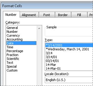
You can format dates and times as you type. For example, if you type 2/2 in a cell, Excel automatically interprets this as a date and displays 2-Feb in the cell. If this isn’t what you want—for example, if you would rather show February 2, 2009 or 2/2/09 in the cell—you can choose a different date format in the Format Cells dialog box, as explained in the following procedure. Similarly, if you type 9:30 a or 9:30 p in a cell, Excel will interpret this as a time and display 9:30 AM or 9:30 PM. Again, you can customize the way the time appears in the Format Cells dialog box.
-
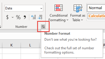
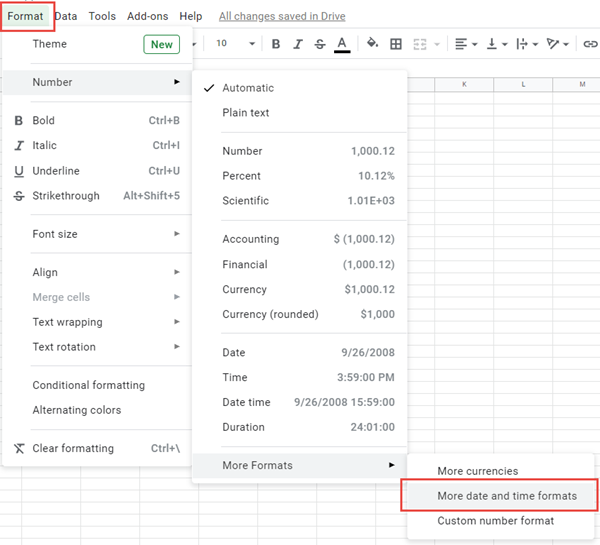
On the Home tab, in the Number group, click the Dialog Box Launcher next to Number.

You can also press CTRL+1 to open the Format Cells dialog box.
-
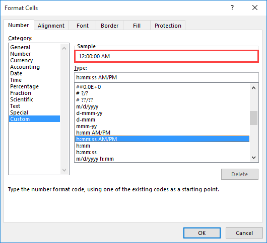
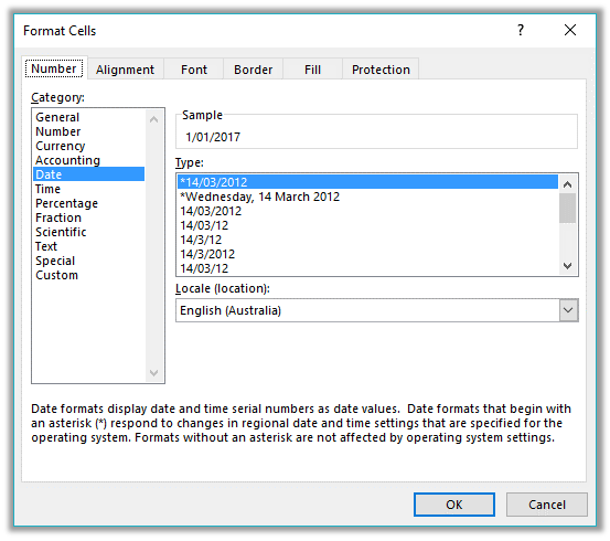
In the Category list, click Date or Time.
-
In the Type list, click the date or time format that you want to use.
Note: Date and time formats that begin with an asterisk (*) respond to changes in regional date and time settings that are specified in Control Panel. Formats without an asterisk are not affected by Control Panel settings.
-
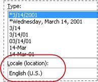
To display dates and times in the format of other languages, click the language setting that you want in the Locale (location) box.
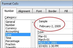
The number in the active cell of the selection on the worksheet appears in the Sample box so that you can preview the number formatting options that you selected.

Top of Page
Create a custom date or time format
-
On the Home tab, click the Dialog Box Launcher next to Number.
You can also press CTRL+1 to open the Format Cells dialog box.
-
In the Category box, click Date or Time, and then choose the number format that is closest in style to the one you want to create. (When creating custom number formats, it’s easier to start from an existing format than it is to start from scratch.)
-
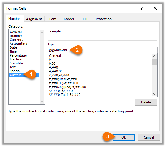
In the Category box, click Custom. In the Type box, you should see the format code matching the date or time format you selected in the step 3. The built-in date or time format can’t be changed or deleted, so don’t worry about overwriting it.
-
In the Type box, make the necessary changes to the format. You can use any of the codes in the following tables:
Days, months, and years
|
To display |
Use this code |
|---|---|
|
Months as 1–12 |
m |
|
Months as 01–12 |
mm |
|
Months as Jan–Dec |
mmm |
|
Months as January–December |
mmmm |
|
Months as the first letter of the month |
mmmmm |
|
Days as 1–31 |
d |
|
Days as 01–31 |
dd |
|
Days as Sun–Sat |
ddd |
|
Days as Sunday–Saturday |
dddd |
|
Years as 00–99 |
yy |
|
Years as 1900–9999 |
yyyy |
If you use «m» immediately after the «h» or «hh» code or immediately before the «ss» code, Excel displays minutes instead of the month.
Hours, minutes, and seconds
|
To display |
Use this code |
|---|---|
|
Hours as 0–23 |
h |
|
Hours as 00–23 |
hh |
|
Minutes as 0–59 |
m |
|
Minutes as 00–59 |
mm |
|
Seconds as 0–59 |
s |
|
Seconds as 00–59 |
ss |
|
Hours as 4 AM |
h AM/PM |
|
Time as 4:36 PM |
h:mm AM/PM |
|
Time as 4:36:03 P |
h:mm:ss A/P |
|
Elapsed time in hours; for example, 25.02 |
[h]:mm |
|
Elapsed time in minutes; for example, 63:46 |
[mm]:ss |
|
Elapsed time in seconds |
[ss] |
|
Fractions of a second |
h:mm:ss.00 |
AM and PM If the format contains an AM or PM, the hour is based on the 12-hour clock, where «AM» or «A» indicates times from midnight until noon and «PM» or «P» indicates times from noon until midnight. Otherwise, the hour is based on the 24-hour clock. The «m» or «mm» code must appear immediately after the «h» or «hh» code or immediately before the «ss» code; otherwise, Excel displays the month instead of minutes.
Creating custom number formats can be tricky if you haven’t done it before. For more information about how to create custom number formats, see Create or delete a custom number format.
Top of Page
Tips for displaying dates or times
-
To quickly use the default date or time format, click the cell that contains the date or time, and then press CTRL+SHIFT+# or CTRL+SHIFT+@.
-
If a cell displays ##### after you apply date or time formatting to it, the cell probably isn’t wide enough to display the data. To expand the column width, double-click the right boundary of the column containing the cells. This automatically resizes the column to fit the number. You can also drag the right boundary until the columns are the size you want.
-
When you try to undo a date or time format by selecting General in the Category list, Excel displays a number code. When you enter a date or time again, Excel displays the default date or time format. To enter a specific date or time format, such as January 2010, you can format it as text by selecting Text in the Category list.
-
To quickly enter the current date in your worksheet, select any empty cell, and then press CTRL+; (semicolon), and then press ENTER, if necessary. To insert a date that will update to the current date each time you reopen a worksheet or recalculate a formula, type =TODAY() in an empty cell, and then press ENTER.
Need more help?
You can always ask an expert in the Excel Tech Community or get support in the Answers community.
Need more help?
How to Format Time in Excel? (Step by Step)
Table of contents
- How to Format Time in Excel? (Step by Step)
- Understanding the Time Format Code
- Different Formatting Technique for More than 24 Hours’ Time
- Things to Remember
- Recommended Articles
As we know, we can apply the time format for any decimal or fractional value.

Now, let us learn how to use the time format in Excel for the 0.25 value.
- We must first select the cell. Then, right-click and choose FORMAT Cell excel.

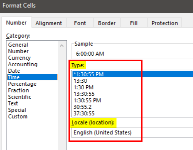
- Now, we can see below the Format Cells window. From there, choose the Time category.

- Now, we can see all the time types available for this value as per the location setting.

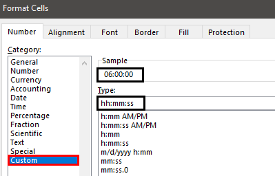
- We can see the preview of the selected cell time format. Choose any of the ones to see a similar time in the cell.

- Using the Time format category, we can also use the Custom category to modify the time format.

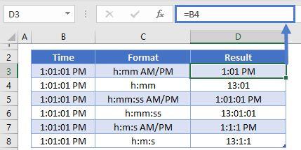
- We have applied the formatting code as hh:mm:ss, so our time shows the preview as 06:00:00. This time format code will show the time in 24-hour format. So if we do not want to see the 24-hour time format, we must enter the AM / PM separator.


So, this will differentiate the “AM” and “PM” times.
Understanding the Time Format Code
As we learned, the Excel time format code is hh:mm:ss. Let me explain this code in detail now.
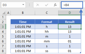
- hh: This time code represents the hour part of the time in double-digit value. For example, in the above example, our time value showed as “06.” If we mention a single “h,” the hour part will be only “6,” not “06.”
- mm: This code represents a minute part of the time in a double-digit value.
- ss: This will represent the second part of the time.
If we do not want to see the “seconds” part from the time, then apply only the “time and minute” part of the code.

We can also customize the time. For example, “0.689” equals the time of “04:32:10 PM.”

So, instead of showing like the below, we can modify it as “04 Hours, 32 Minutes, 10 Seconds”.

We get the following result.

For this, we must enter the below custom time code.
hh “hours”, mm “Minutes”, ss “Seconds” AM/PM
So, this will display the time as we have shown above.
Different Formatting Techniques for More than 24 Hours
Working with time could be tricky if we do not know the full formatting technique because if we want to enter the time more than 24 hours, we need to employ a different formatting code.
For example, Mr. A was a sales manager. Below are his call records for the past five days.
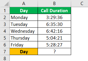
Now, he wants to calculate his total call duration for the week.

So, let us sum all the days in the time format of cell B7.

We got the total as “03:20:10,” which is wrong.
It is a real-time experience. Looking at the data, we can easily say the total duration is more than “03:20:10,” so what is its issue?
The issue is when the summation or time value exceeds 24 hours, we need to give slightly different time formatting codes.
For example, let us select the call duration time and see the status barAs the name implies, the status bar displays the current status in the bottom right corner of Excel; it is a customizable bar that can be customized to meet the needs of the user.read more to see the sum of the values chosen.

So, the total in the status bar is “27:20:10,” but our SUM functionThe SUM function in excel adds the numerical values in a range of cells. Being categorized under the Math and Trigonometry function, it is entered by typing “=SUM” followed by the values to be summed. The values supplied to the function can be numbers, cell references or ranges.read more has returned “03:20:10.”
To understand this better, we must copy the result cell and use paste specialPaste special in Excel allows you to paste partial aspects of the data copied. There are several ways to paste special in Excel, including right-clicking on the target cell and selecting paste special, or using a shortcut such as CTRL+ALT+V or ALT+E+S.read more as values in another cell.

We get the value as 1.13900463. i.e., 1 Day, 20 minutes, 10 seconds.
As we told you, the time value is stored as serial numbers from 0 to 0.9999; we are getting this error sum since this total is crossing the fraction mark.
So for this, we need to apply the time formatting code as “[hh]:mm:ss.”

We get the following result.

Same formula, we have changed the time format to [hh]:mm:ss.
Things to Remember
- Time is stored as decimal values in Excel.
- The date and time are combined in Excel.
- When the time value exceeds 24 hours, we must enclose the time format code of the hour part inside the parenthesis, “[hh]:mm:ss.”
Recommended Articles
This article is a guide to formatting time in Excel. We discuss formatting time in Excel with practical examples and downloadable Excel templates. You can learn more from the following articles: –
- Format Text in Excel
- Add Time in Excel
- TimeValue in VBA
- Subtract Time in Excel
In Excel, working with the time is not difficult but you need to know a few rules to avoid big mistakes. In this article you will learn these rules and how to manage time formats.
Difference between date and time in Excel
In Excel, hours are always a fraction of a day. So it is necessarily decimal numbers.
This rule is fundamental to avoid mistakes in calculation and display.
- Dates are whole numbers (like 1, 2, 3, ….)
- Hours are decimal numbers (like 0.5, 0.33333, …)
A whole number will never be understood as hours or minutes in a worksheet ❗❗❗
A very good example of used is the technique to split date and time to 2 different cells.

Why I can’t convert to Time format
For instance, in this situation, you have whole number in column A. But when you apply the Time format, all the cells returned 00:00:00 🤔

But this is absolutely normal. In Excel, a whole number is a day (and not a time). Now, if you convert to Date & Time format you have this result

How to Convert a whole number in Time
If you have to convert a whole number to Time, you must divide that number by 24 (the number of hours in a day 😉).
=8/24 = 0,333333

Then, you apply the Time format, you have the correct result 😍😎

If the content of your cell is a seconde and not hour, then the formula is
=8/(24*60*60)
Technique with Paste Special — Divide
DON’T waste your time. There is a technique to divide all your numbers by 24 in 2 steps.
The secret is to use paste special (option divide) 😍😍😍
Time format hours, minutes and seconds

In the article Date Format, we saw how to customize the date and time using the dialog box Number Format.
To customize a time, you use the following parameters.
- h for the hour
- m for the minute
- s for the second
Hours over 24 hours
By default in Excel, Time values is between 00:00:00:and 23:59:59
But there is a trick to display times over 24 hours 😉

Tenth, hundredth, thousandth
You can also display the tenth, hundredth and thousandth. But for that, you have to add 0.

Skip to content
Вы узнаете об особенностях формата времени Excel, как записать его в часах, минутах или секундах, как перевести в число или текст, а также о том, как добавить время с помощью комбинации клавиш или вставить автоматически обновляемое время с помощью функции СЕЙЧАС. Вы также узнаете, как применять специальные функции времени для получения часов, минут или секунд из значения времени.
Microsoft Excel имеет ряд полезных функций управления временем, и их умение правильно их использовать может сэкономить вам много сил и нервов. Используя функции времени, вы можете вставить текущую дату и время в любом месте рабочего листа, преобразовать время в десятичное число, суммировать различные интервалы времени или вычислить истекшее время.
Чтобы иметь возможность использовать функции времени, полезно знать, как Microsoft Excel хранит время. Итак, прежде чем углубляться в формулы, давайте потратим пару минут на изучение основ форматирования времени в Excel.
Формат времени в Excel
Если вы читали наши статьи по датам в Excel, вы знаете, что Microsoft Excel хранит даты в виде последовательных чисел, начиная с 1 января 1900 года, которое считается как 1. Поскольку время рассматривается как часть дня, то время хранится в виде десятичной дроби.
Во внутренней системе Excel:
- 00:00:00 сохраняется как 0.0
- 23:59:59 сохраняется как 0,99999
- 06:00 — как 0,25
- 12:00 – соответствует 0,5.
Когда в Excel вводятся и дата, и время, они сохраняются в виде десятичного числа, состоящего из целой части, означающей дату (номер дня), и десятичной дроби, представляющей время. Например, 1 сентября 2022 г., 13:00:00 хранится как 44805,5416666667.
Формат времени по умолчанию в Excel
При изменении формата времени в диалоговом окне «Формат ячеек» вы видите список возможных шаблонов отображения, первый из которых является форматом по умолчанию.

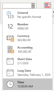
Чтобы быстро применить формат времени по умолчанию к выбранной ячейке или диапазону, щелкните стрелку раскрывающегося списка в группе «Число» на вкладке «Главная» и выберите «Время» .

Чтобы изменить формат времени по умолчанию, перейдите в Панель управления и нажмите Часы и регион > Изменение форматов даты, времени и чисел.
Далее определите, как будет выглядеть краткое и полное время.

Примечание. При создании нового формата времени или изменении существующего помните, что независимо от того, как вы выбрали отображение времени, Excel всегда сохраняет время одним и тем же способом — в виде десятичных чисел.
Перевод времени в десятичное число
Быстрый способ показать число, представляющее определенное время, — использовать диалоговое окно «Формат ячеек».
Просто выберите ячейку, содержащую время, и нажмите Ctrl + 1, чтобы открыть уже знакомое нам диалоговое окно. На вкладке «Число» выберите «Общий» в разделе «Числовые форматы», и вы увидите десятичную дробь в поле «Образец».
Такой перевод времени в число вы видите на скриншоте ниже.

Теперь вы можете записать это число и нажать «Отмена», чтобы закрыть окно и ничего не менять. Или вы можете нажать кнопку OK и представить время соответствующим десятичным числом. Фактически, вы можете считать это самым быстрым, простым и без применения формул способе перевести время в десятичное число в Excel.
Далее мы более подробно рассмотрим специальные функции времени и приёмы для преобразования времени в часы, минуты или секунды.
Как применить или изменить формат времени
Microsoft Excel достаточно умен, чтобы распознавать время прямо в процессе ввода и «на лету» соответствующим образом отформатировать ячейку. Например, если вы введете 10:30, то программа сразу поймет, что это, и отобразит как число в виде времени, а не просто как текст.
Если вы хотите отформатировать какие-то числа как время или применить другой способ отображения времени к уже существующим значениям времени, вы можете сделать это с помощью диалогового окна «Формат ячеек», как описано ниже.
- На рабочем листе выберите ячейки, к которым вы хотите применить или в которых нужно изменить представление времени.
- Откройте диалоговое окно «Формат ячеек», нажав Ctrl + 1 или щелкнув значок диалогового окна форматов на вкладке главного меню.

- На вкладке «Число» выберите «Время» и укажите подходящий вам вариант в поле «Тип».
- Нажмите OK, чтобы применить выбранный формат времени и закрыть диалоговое окно.

Создание пользовательского формата времени
Хотя Microsoft Excel предоставляет несколько различных шаблонов отображения времени, вы можете создать свой собственный, который лучше всего подходит именно для вас. Для этого откройте окно «Формат ячеек», выберите «Пользовательский» и введите шаблон времени, который вы хотите применить, в поле «Тип».

Совет. Самый простой способ создать собственный формат времени в Excel — использовать один из уже существующих в качестве отправной точки. Для этого выберите Время в списке и укажите один из предустановленных шаблонов, который ближе всего к желаемому. После этого сразу переключитесь на «Все форматы» и просто внесите изменения в тот шаблон, который будет показан в поле Тип.
При создании пользовательского формата времени вы можете использовать следующие коды.
| Код | Описание | Отображается как |
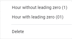
| ч | Часы без ведущего нуля | 0:33 |
| чч | Часы с ведущим нулем | 00:15 |
| м | Минуты без ведущего нуля | 0-59 |
| мм | Минуты с ведущим нулем | 00:59 |
| с | Секунды без ведущего нуля | 0-59 |
| сс | Секунды с ведущим нулем | 00-59 |
В следующей ниже таблице приведены несколько примеров того, как могут выглядеть ваши форматы времени Excel, в том числе вместе с датой:
| Формат времени | Отображается как |
| ч:мм:сс | 19:15:00 |
| ч:мм | 19:15 |
| [$-ru-RU-x-genlower]ДД ММММ ГГГГ г. ч:мм; @ | 26 сентября 2022г. 19:15 |
| дддд ДД ММММ ГГГГ г. ч:мм:сс; @ | Понедельник 26 сентябрь 2022г. 19:15:00 |
Пользовательские форматы для временных интервалов более 24 часов
Может так случиться, что сумма времени превысит 24 часа. Например, нам нужно просуммировать отработанное за месяц время. Чтобы Microsoft Excel правильно отображал время, превышающее 24 часа, примените один из следующих настраиваемых форматов времени.
| Формат времени | Отображается как | Объяснение |
|---|---|---|
| [ч]:мм | 51:30 | 51 час 30 минут |
| [ч]:мм:сс | 51:30:50 | 51 час 30 минут 50 секунд |
| [ч] » час «, мм » мин «, сс » сек» | 51 час 30 мин 50 сек | |
| д ч:мм:сс | 3 3:30:50 | 3 дня, 3 часа , 30 минут и 50 секунд |
| д «дн.» ч:мм:сс | 3 дн. 3:30:50 | |
| д «дн.», ч » час «, м » мин. и » с » сек. « | 3 дн., 3 час , 30 мин. и 50 сек. |
Формат для отрицательных значений времени
Пользовательские форматы времени, рассмотренные выше, работают только для положительных значений. Если результатом ваших вычислений является отрицательное значение (например, когда вы вычитаете большее время из меньшего), то результат будет отображаться как ########. Если вы хотите всё же показать отрицательное время, то есть следующие варианты:
- Отображать пустую ячейку для отрицательного времени. Введите точку с запятой в конце формата времени, например [ч]:мм;
- Отображение сообщения об ошибке. Введите точку с запятой в конце формата, а затем укажите желаемое сообщение в кавычках, например [ч]:мм;»Отрицательное время»
Если вспомнить общие принципы построения форматов в Excel, то точка с запятой действует как разделитель, отделяющий формат положительных значений от способа представления отрицательных значений.
- Если вы хотите отображать отрицательное время со знаком «минус», например -19:30, то самый простой способ для этого — изменить систему дат Excel на систему дат «1904 год». Для этого нажмите « Файл» > «Параметры» > «Дополнительно », прокрутите список вниз и установите флажок «Использовать систему дат 1904».

Нажмите OK , чтобы сохранить новые настройки, и теперь отрицательные величины времени будут отображаться так же, как и как отрицательные числа:

Также отрицательное время можно отобразить при помощи формул. Как использовать для этого текстовый формат времени – читайте в разделе Как рассчитать и отобразить отрицательное время в Excel.
Как вставить текущее время в Excel
Существует несколько способов вставки времени в Excel, какой из них использовать, зависит от того, хотите ли вы зафиксировать какой-то момент времени или иметь динамическое значение, которое автоматически обновляется, чтобы показать текущее время.
Как добавить неизменяемое значение времени
Если вы ищете способ вставить метку времени, т. е. статическое значение, которое не будет автоматически обновляться при пересчете рабочей книги, используйте один из следующих способов:
- Чтобы вставить текущее время , нажмите
Ctrl + Shift + 6 - Чтобы ввести текущую дату и время , нажмите
Ctrl + Shift + 4что позволит вставить дату, затем нажмитеПробел, и после этого задействуйте комбинациюCtrl + Shift + 6, чтобы вставить текущее время.

Добавьте сегодняшнюю дату и текущее время, используя функцию ТДАТА
Если вы хотите вставить текущую дату и время в качестве динамического значения, которое обновляется автоматически, используйте функцию Excel ТДАТА.
Формула настолько проста, насколько это возможно, и никаких аргументов не требуется:
=ТДАТА()
При использовании функции ТДАТА следует помнить о нескольких вещах:
- Функция ТДАТА извлекает время из системных часов вашего компьютера.
- Это одна из изменчивых функций, которая заставляет формулу пересчитываться каждый раз, когда рабочий лист повторно открывается или в нем изменяется хотя бы одно значение.
- Чтобы заставить функцию ТДАТА обновить значение даты и времени, нажмите либо
Shift + F9для пересчета активного рабочего листа илиF9для пересчета всех открытых книг. - Чтобы показать только время, установите нужный вам формат времени, как описано выше.
Помните, что это изменит только внешний вид, а фактическое значение по-прежнему будет десятичным числом, состоящим из целой части, представляющей дату, и дробной части, представляющей время.
Чтобы в ячейке осталось действительно только значение времени, используйте следующую формулу:
=ТДАТА() — ЦЕЛОЕ(ТДАТА())
Функция ЦЕЛОЕ используется для округления десятичного числа, возвращаемого ТДАТА(), до ближайшего целого. А затем вы из даты-времени вычитаете целую часть, представляющую сегодняшнюю дату, чтобы оставить только дробную часть, то есть текущее время.
Поскольку формула возвращает десятичное число, вам также нужно будет применить формат времени, чтобы значение отображалось правильно.
Как вставить текущую дату и время как неизменяемую метку времени
Очень часто у пользователей возникает вопрос: «Какую формулу мне использовать для ввода времени в моем листе Excel, чтобы оно не менялось каждый раз, когда рабочий лист повторно открывается или пересчитывается?»
Первый способ – это использование комбинации клавиш, о которой мы говорили чуть выше.
Второй способ – используйте функцию ТДАТА. Затем скопируйте полученное значение в буфер обмена при помощи комбинации клавиш CTRL+C или через контекстное меню по правой кнопке мыши.
После это вставьте скопированное значение (не формулу!) в эту же ячейку, используя меню «Специальная вставка» — «Вставить значения». Либо поможет комбинация клавиш CTRL + ALT + V. Формула будет заменена статическим значением даты и времени.
Третий способ. Для начала я хотел бы отметить, что я не могу на 100% рекомендовать это решение, потому что оно включает циклические ссылки, а к ним следует относиться с большой осторожностью.
Во всяком случае, вот что можно сделать…
Допустим, у вас есть список товаров в столбце А, и как только определенный товар будет отправлен покупателю, вы вводите «Да» в столбце «Доставка», то есть в столбце В. Как только там появится «Да», вы хотите автоматически вставить текущую дату и время в ту же строку в столбце C и сделать так, чтобы эта отметка времени уже не менялась. Согласитесь, если товаров много, то вручную вводить дату и время будет весьма утомительно. Даже с использованием комбинации клавиш, о чем мы говорили чуть выше. Поэтому этот процесс желательно автоматизировать.
Для этого мы попробуем использовать следующую вложенную формулу ЕСЛИ с циклическими ссылками во второй функции ЕСЛИ:
=ЕСЛИ(B2=»да»; ЕСЛИ(C2=»»; ТДАТА(); C2); «»)
Где B — столбец «Доставка», а C2 — ячейка, в которую вы вводите формулу и где в конечном итоге появится значение времени.

В приведенной выше формуле первая функция ЕСЛИ проверяет B2 на наличие слова «Да» (или любого другого текста, который вы указываете в формуле), и если указанный текст присутствует, то она выполняет вторую функцию ЕСЛИ. В противном случае – просто возвращает пустую строку.
А вот второе ЕСЛИ — это циклическая формула, которая заставляет функцию СЕЙЧАС возвращать в С2 текущий день и время, если там еще нет никакого значения.
Если вместо проверки какого-либо конкретного слова вы хотите, чтобы временная метка появлялась, когда вы помещаете что-либо в указанную ячейку (это может быть любое число, текст или дата), тогда используйте первую функцию ЕСЛИ для проверки непустой ячейки:
=ЕСЛИ(B2<>»»; ЕСЛИ(C2=»»; ТДАТА(); C2); «»)
Примечание. Если ячейка ссылается сама на себя, то возникает так называемая циклическая ссылка.
Вот очень точное и краткое определение циклической ссылки, предоставленное Microsoft:
» Когда формула Excel прямо или косвенно ссылается на собственную ячейку, она создает циклическую ссылку. «
Вычисления как бы идут по кругу непрерывно. Возникает замкнутый цикл, Excel все время занят расчетом этой формулы. И если формула достаточно сложная, то это может привести к существенному снижению производительности и скорости расчетов.
Поэтому использование циклических ссылок в Excel — скользкий и не рекомендуемый подход. Помимо проблем с производительностью и предупреждающего сообщения, отображаемого при каждом открытии книги (если не включены итерационные вычисления), циклические ссылки могут привести к ряду других проблем, которые не сразу бросаются в глаза.
Например, если вы выбрали ячейку с циклической ссылкой, а затем случайно переключились в режим редактирования формулы (либо нажатием F2, или двойным кликом по ячейке), а затем нажмете Enter, не внося никаких изменений в формулу, то она вернет ноль.
Поэтому по возможности старайтесь избегать циклических ссылок в своих таблицах. И если идёте на их применение, то делайте это осознанно.
Чтобы циклическая формула Excel работала, вы должны разрешить итерационные вычисления на своем листе.
Говоря простым языком, итерация – это повторяющийся пересчет формулы. Итерационные вычисления обычно отключены в Excel по умолчанию. Это сделано для того, чтобы формулы с циклическим ссылками не работали. Чтобы в текущей рабочей книге разрешить расчет циклических формул, нужно сделать следующее.
В меню Файл > Параметры , перейдите к Формулы и установите флажок Включить итеративный расчет в разделе Параметры расчета.

При включении итерационных вычислений необходимо указать следующие два параметра:
- Поле «Максимум итераций» — указывает, сколько раз формула должна пересчитываться. Чем больше число итераций, тем больше времени занимает расчет.
- Поле «Максимальное изменение» — указывает максимальное изменение между результатами расчета. Чем меньше число, тем более точный результат вы получите и тем больше времени потребуется для расчета рабочего листа.
Значения по умолчанию: 100 для максимального количества итераций и 0,001 для максимального изменения . Это означает, что Microsoft Excel прекратит вычисление вашей циклической формулы после 100 итераций или после изменения менее 0,001 между итерациями, в зависимости от того, что наступит раньше.
В итоге ваша формула для вставки текущей даты будет выполнена 100 раз, после чего дата всё же будет вставлена в пустую ячейку. Существенного влияния на производительность это не окажет.
Но обо всех возможных негативных последствиях использования циклических ссылок вам все же не следует забывать.
Как вставить нужное время
Функция ВРЕМЯ используется для преобразования значений, показывающих часы, минуты и секунды, в десятичное число, представляющее время.
Синтаксис её очень прост:
=ВРЕМЯ(часы; минуты; секунды)
Аргументы часы, минуты и секунды могут быть указаны в виде чисел от 0 до 32767.
- Если часы больше 23, он делится на 24, а остаток принимается за значение часа.
Например, ВРЕМЯ(30, 0, 0) то же самое, что ВРЕМЯ(6,0,0), что даст результат 0,25 или 6:00.
- Если аргумент минуты больше 59, они преобразуются в часы и минуты. И если секунды больше 59, они автоматически преобразуются в часы, минуты и секунды.
Например, ВРЕМЯ(0, 930, 0) преобразуется в ВРЕМЯ(15, 30, 0), что составляет 0,645833333 или 15:30.
Функция ВРЕМЯ полезна, когда речь идет об объединении отдельных значений в одно значение времени. Например значений отдельных единиц времени, записанными в других ячейках или возвращаемых другими функциями.

Как получить часы, минуты и секунды из значения времени
Чтобы извлечь единицы времени из значения времени, вы можете использовать следующие функции времени Excel:
ЧАС(время) — возвращает час значения времени в виде целого числа от 0 (00:00) до 23 (23:00).
МИНУТЫ(время) — получает минуты значения времени в виде целых чисел от 0 до 59.
СЕКУНДЫ(время) — возвращает секунды значения времени в виде целых чисел от 0 до 59.
Во всех трех функциях вы можете вводить время в виде текстовых строк, заключенных в двойные кавычки (например, «6:00»), в виде десятичных чисел (например, 0,25, что представляет 6:00) или в виде результатов других функций. Несколько примеров формул следуют ниже.
- =ЧАС(A2)— возвращает часы метки времени из A2.
- =МИНУТЫ(A2)— возвращает минуты из A2.
- =СЕКУНДЫ(A2)— возвращает секунды.
- =ЧАС(ТДАТА())— возвращает текущий час.

Как отобразить время больше чем 24 часа, 60 минут, 60 секунд
Чтобы отобразить интервал времени более 24 часов, 60 минут или 60 секунд, примените пользовательский формат времени, в котором соответствующий код единицы времени заключен в квадратные скобки, например [ч], [м] или [с].
Вот простое пошаговое руководство:
- Выберите ячейки, которые вы хотите отформатировать.
- Щелкните правой кнопкой мыши выбранное и нажмите
Ctrl + 1. Это откроет диалоговое окно «Формат ячеек». - На вкладке «Число» выберите «Пользовательский» и введите один из следующих шаблонов времени в поле «Тип».
- Более 24 часов: [ч]:мм:сс или [ч]:мм
- Более 60 минут: [м]:сс
- Более 60 секунд: [с]
На скриншоте ниже показан пользовательский формат времени «более 24 часов» в действии:

Ниже есть примеры нескольких других пользовательских форматов, которые можно использовать для отображения временных интервалов, превышающих длину стандартных единиц времени.
| Описание | Код |
| Все часы | [ч] |
| Часы и минуты | [ч]:мм |
| Часы, минуты, секунды | [ч]:мм:сс |
| Всего минут | [м] |
| Минуты и секунды | [м]:сс |
| Всего секунд | [с] |
Применительно к нашим примерам данных (общее время 49:30) эти форматы времени дадут следующие результаты:

Чтобы сделать отображаемую информацию более наглядной и понятной для ваших пользователей, можете дополнить временные единицы соответствующими словами, например:

Примечание. Хотя приведенное выше время выглядит как текст, всё же оно по-прежнему является числовым значением. Ведь форматы Excel изменяют только визуальное представление, но не сами значения. Таким образом, вы можете добавлять и вычитать отформатированное время как обычно, ссылаться на него в своих формулах и использовать в других вычислениях.
Теперь, когда вы разобрались с форматом времени Excel и функциями времени, вам будет намного проще работать с датами и временем в ваших таблицах.
 Как перевести время в число — В статье рассмотрены различные способы преобразования времени в десятичное число в Excel. Вы найдете множество формул для преобразования времени в часы, минуты или секунды. Поскольку Microsoft Excel использует числовую систему для работы с временем, вы можете…
  Как вывести месяц из даты — На примерах мы покажем, как получить месяц из даты в таблицах Excel, преобразовать число в его название и наоборот, а также многое другое. Думаю, вы уже знаете, что дата в…
 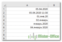 Как быстро вставить сегодняшнюю дату в Excel? — Это руководство показывает различные способы ввода дат в Excel. Узнайте, как вставить сегодняшнюю дату и время в виде статической метки времени или динамических значений, как автоматически заполнять столбец или строку…
 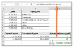 Количество рабочих дней между двумя датами в Excel — Довольно распространенная задача: определить количество рабочих дней в период между двумя датами – это частный случай расчета числа дней, который мы уже рассматривали ранее. Тем не менее, в Excel для…
Return to Excel Formulas List
Download Example Workbook
Download the example workbook
This tutorial will demonstrate how to change time formats in Excel and Google Sheets.
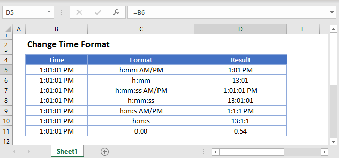
Excel Time Format
In spreadsheets, times are stored as decimal values where each 1/24th represents one hour of a day (Note: Dates are stored as whole numbers, adding a decimal value to a date number will create a time associated with a specific date). When you type a time into a cell, the time is converted to it’s corresponding decimal value and the number format is changed to time.
After a time is entered in Excel as a time, there are several ways to change the formatting:
Change Time Formats
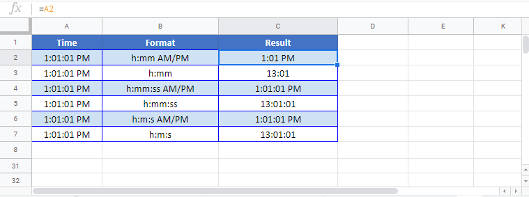
Time Format
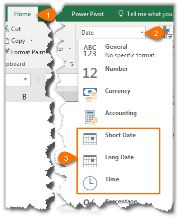
The Ribbon Home > Number menu allows you to change a time to the default Time Format:
Format Cells Menu – Time
The Format Cells Menu gives you numerous preset time formats:
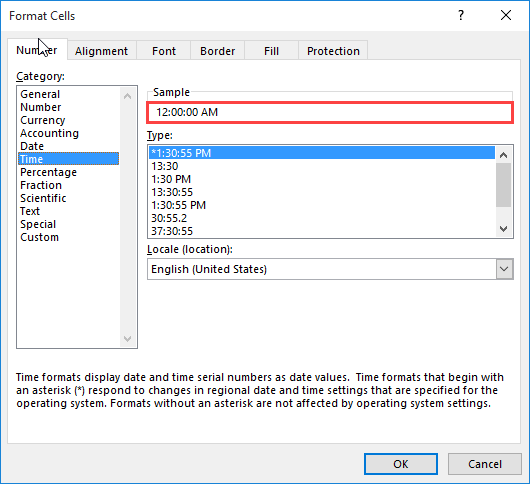
Notice that in the ‘Sample’ area you can see the impact the new number format will have on the active cell.
The Format Cells Menu can be accessed with the shortcut CTRL + 1 or by clicking this button:
Custom Number Formatting
The Custom section of the Format Cells Menu allows you the ability to create your own number formats:
To set custom number formatting for times, you’ll need to specify how to display hours, minutes, and/or seconds. Use this table as guide:
You can use the above examples to only display hours, minutes, or seconds. Or you can combine them to form a complete time:
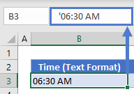
Times Stored as Text
Time as Text
To store a time as text, type an apostrophe (‘) in front of the time as you’re typing it:
However, as long as the time is stored as text you’ll be unable to change the formatting like a normal time.
You can convert the time stored as text, back to a time using the TIMEVALUE or VALUE Functions:
=TIMEVALUE(B3)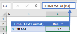
Text Function
The TEXT Function is a great way to display a time as text. The TEXT Function allows you to display times in formats just like the Custom Number Formatting discussed previously.
=TEXT(B3,C3)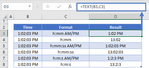
You can combine the TEXT Function with a string of text like this:
="Current time is: "&TEXT(NOW(),"h:mm:ss AM/PM")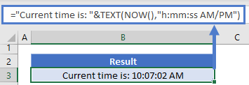
Google Sheets Date Formatting
Google Sheets makes formatting times slightly easier. With Google Sheets, you simply need to navigate to the ‘More date and time formats’:
The menu looks like this:

You’ll be able to select from a wide range of presets. Or you can utilize the drop-downs on top to select your desired format:
In Google Sheets your formatted time will look like this:
Even though dates and time are actually stored as a regular number known as the date serial number, we can make use of extensive Excel date and time formatting options to display them just the way we want.
We can access some quick date and time formats from the Home tab > in the Number group:
We can also create our own custom date and time formats to suit our needs. Let’s take a look.
- Select the cell(s) containing the dates you want to format.
- Press CTRL+1, or right-click > Format Cells to open the Format Cells dialog box.
- On the Number tab select ‘Date’ in the Categories list. This brings up a list of default date formats you can select from in the ‘Type’ list. Likewise for the Time category.
We aren’t limited to the defaults though. You can create your own Custom date or time formats in the ‘Custom’ category. These custom formats are saved for you to re-use in the current file.
Custom Date Formatting Characters
Excel recognises the following characters and sets of characters for date formatting.
| Character | Explanation | Date | Formatted | |
| d | Displays the day as a number without a leading zero. | 3/09/2016 | 3 | |
| dd | Displays the day as a number with a leading zero when appropriate. | 3/09/2016 | 03 | |
| ddd | Displays the day as an abbreviation (Sun to Sat). | 3/09/2016 | Sat | |
| dddd | Displays the day as a full name (Sunday to Saturday). | 3/09/2016 | Saturday | |
| m | Displays the month as a number without a leading zero. | 3/09/2016 | 9 | |
| mm | Displays the month as a number with a leading zero when appropriate. | 3/09/2016 | 09 | |
| mmm | Displays the month as an abbreviation (Jan to Dec). | 3/09/2016 | Sep | |
| mmmm | Displays the month as a full name (January to December). | 3/09/2016 | September | |
| mmmmm | Displays the month as a single letter (J to D). | 3/09/2016 | S | |
| yy | Displays the year as a two-digit number. | 3/09/2016 | 16 | |
| yyyy | Displays the year as a four-digit number. | 3/09/2016 | 2016 |
Custom Date Formatting Examples
We can bring the characters together to create our own custom formats. Some examples below:
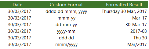
Remember; the custom format doesn’t alter the underlying date serial number, it is still the same.
Custom Time Formatting Characters
Like dates, time also has its own set of custom formatting characters, as listed below:
| Character | Explanation | ||
| h | Displays the hour as a number without a leading zero. | ||
| [h] | Displays elapsed time in hours. If you are working with a formula that returns a time in which the number of hours exceeds 24, use a number format that resembles [h]:mm:ss or [h]:mm | ||
| hh | Displays the hour as a number with a leading zero when appropriate. If the format contains AM or PM, the hour is based on the 12-hour clock. Otherwise, the hour is based on the 24-hour clock. | ||
| m | Displays the minute as a number without a leading zero.* | ||
| [m] | Displays elapsed time in minutes. If you are working with a formula that returns a time in which the number of minutes exceeds 60, use a number format that resembles [mm]:ss. | ||
| mm | Displays the minute as a number with a leading zero when appropriate.* | ||
| s | Displays the second as a number without a leading zero. | ||
| [s] | Displays elapsed time in seconds. If you are working with a formula that returns a time in which the number of seconds exceeds 60, use a number format that resembles [ss]. | ||
| ss | Displays the second as a number with a leading zero when appropriate. If you want to display fractions of a second, use a number format that resembles h:mm:ss.00. | ||
| AM/PM, am/pm, A/P, a/p | Displays the hour using a 12-hour clock. Excel displays AM, am, A, or a for times from midnight until noon and PM, pm, P, or p for times from noon until midnight. |
*Note: The m or mm code must appear immediately after the h or hh code or immediately before the ss code; otherwise, Excel displays the month instead of minutes.
Custom Time Formatting Examples
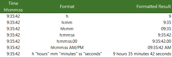
Note: if your PC region settings have the Date & Time formats set to show the Short Time as hh:mm tt or the Long Time as hh:mm:ss tt then this may override any single ‘h’ formats and display them as ‘hh’.
The screenshot above is what I see with my PC region settings for the Short Time as h:mm tt. If you see something different when using a single ‘h’ format, then it will be down to your PC region settings.
More Excel Formatting
Custom cell formatting isn’t limited to dates and times. There is a plethora of formatting options for all types of numbers that we can use to get our reports looking just the way we want. Click here for our comprehensive guide to Excel custom number formatting.
Free eBook — Working with Date & Time in Excel
Everything you need to know about Date and Time in Excel — Download the free eBook and Excel file with detailed instructions.
Enter your email address below to download the comprehensive Excel workbook and PDF.
By submitting your email address you agree that we can email you our Excel newsletter.
Transcript
In this lesson we’ll look at the Time format. Like the Date format, the Time format includes a number of built-in options for displaying time.
Let’s take a look.
Here we have a set of times in column B of our table. Let’s start off by copying these times to all columns, then adjust formats to match those shown in the table header.
Let’s look first at the default time format in column C. This is the format you get when you apply the Time format using the menu in the ribbon.
If we check this format in the Format Cells dialog, we see it listed first, with an asterisk.
The asterisk means that this time format is controlled by the regional settings on the computer.
If we change the time format in Windows, in the Region and Language control panel, we’ll see the change in Excel for cells that use this time format.
This means that this time format may look different on different computers, depending on regional settings. If you need to ensure that the display of time is always the same, it’s better to use another format option.
To set the time format indicated in columns D through H, we need to use the Format Cells dialog.
We can set time to display in military format—without the AM or PM—with and without seconds.
We can also use Format Cells to show a standard AM/PM time with and without seconds.
Finally, we have the option to select a time format that includes a date. Because these times don’t contain a date component, Excel will display the first date in its date system. As a result, time formats that include a date only make sense when the cell contains both a date and a time.
MS Excel offers many possibilities how display date and time. The custom format can be set in the Format Cells… menu. Do the right-click and select Format Cells… .

In the item Number select Custom.

Into the field Type: write the date/time codes.
Date format codes
Day
d – day number (0–31)
dd – day number (01–31) / two digits
ddd – day as an abbreviation (mon–sun)
dddd –day name (monday–sunday)
Month
m – month number (1–12)
mm – month number (01–12) / two digits
mmm –month as an abbreviation (Jan–Dec)
mmmm – month name (January–December)
mmmmm – the first letter of month name
Year
yy – year number (00–99) / two digits
yyyy – year number (1900–9999) / four digits
Examples of custom date format
Let’s have the date 3.1.2012
| Code | Date |
| dd/mm/yyyy | 03/01/2012 |
| mm/dd/yyyy | 01/03/2012 |
| d-m-yyyy | 3-1-2012 |
| dd-mm-yy | 03-01-12 |
| dddd | Tuesday |
| dd. mm. yyyy dddd | 03. 01. 2012 Tuesday |
| mmmm | January |
| d. mmmm yyyy | 3. January 2012 |
| mmmm dd, yyyy | January 03, 2012 |
| dddd, mmmm dd yyyy | Tuesday, January 03 2012 |
| ddmmyy | 030112 |
| dd. “text” | 03. text |
Time format codes
h – hour number (0–23)
hh – hour number (00–23) / two digits
m – minute number (0–59)
mm – minute number (00–59)
s – second number (0–59)
ss – second number (00–59)
AM/PM or am/pm – Convert from 24 Hour to 12 Hour Time
[h] – elapsed time in hours (can be greater than 24, e.g. for sports results)
[mm] – elapsed time in minutes (can be greater than 60, e.g. for sports results)
[ss] – elapsed time in minutes (can be greater than 60, e.g. for sports results)
h:mm:ss.00 – fractions of seconds
Examples of custom time format
Let’s have the time 6:25:31
| Code | Time |
| hh.mm | 06.25 |
| hhmm | 0625 |
| h:mm:ss AM/PM | 6:25:31 am |
| hh “hours and” mm “minutes” | 06 hours and 25 minutes |
| [m] | 385 (the number of minutes since 00:00:00) |
| [s] | 23131 (the number of seconds since 00:00:00) |
Examples of custom date/time format
Date and time formats can be combined. Notice that month and minute have the same code. Immediately after the hours writes Excel the minutes.
Default date/time: 4.11.2010 6:25
| Code | Date/Time |
| hh:mm dd/mm/yyyy | 06:25 04/11/2012 |
| dddd hh:mm | Thursday 06:25 |
Note: In other language versions of Excel can be format codes different.