
Formatting Cells Number
General
Range("A1").NumberFormat = "General"Number
Range("A1").NumberFormat = "0.00"Currency
Range("A1").NumberFormat = "$#,##0.00"Accounting
Range("A1").NumberFormat = "_($* #,##0.00_);_($* (#,##0.00);_($* ""-""??_);_(@_)"Date
Range("A1").NumberFormat = "yyyy-mm-dd;@"Time
Range("A1").NumberFormat = "h:mm:ss AM/PM;@"Percentage
Range("A1").NumberFormat = "0.00%"Fraction
Range("A1").NumberFormat = "# ?/?"Scientific
Range("A1").NumberFormat = "0.00E+00"Text
Range("A1").NumberFormat = "@"Special
Range("A1").NumberFormat = "00000"Custom
Range("A1").NumberFormat = "$#,##0.00_);[Red]($#,##0.00)"Formatting Cells Alignment
Text Alignment
Horizontal
The value of this property can be set to one of the constants: xlGeneral, xlCenter, xlDistributed, xlJustify, xlLeft, xlRight.
The following code sets the horizontal alignment of cell A1 to center.
Range("A1").HorizontalAlignment = xlCenterVertical
The value of this property can be set to one of the constants: xlBottom, xlCenter, xlDistributed, xlJustify, xlTop.
The following code sets the vertical alignment of cell A1 to bottom.
Range("A1").VerticalAlignment = xlBottomText Control
Wrap Text
This example formats cell A1 so that the text wraps within the cell.
Range("A1").WrapText = TrueShrink To Fit
This example causes text in row one to automatically shrink to fit in the available column width.
Rows(1).ShrinkToFit = TrueMerge Cells
This example merge range A1:A4 to a large one.
Range("A1:A4").MergeCells = TrueRight-to-left
Text direction
The value of this property can be set to one of the constants: xlRTL (right-to-left), xlLTR (left-to-right), or xlContext (context).
The following code example sets the reading order of cell A1 to xlRTL (right-to-left).
Range("A1").ReadingOrder = xlRTLOrientation
The value of this property can be set to an integer value from –90 to 90 degrees or to one of the following constants: xlDownward, xlHorizontal, xlUpward, xlVertical.
The following code example sets the orientation of cell A1 to xlHorizontal.
Range("A1").Orientation = xlHorizontalFont
Font Name
The value of this property can be set to one of the fonts: Calibri, Times new Roman, Arial…
The following code sets the font name of range A1:A5 to Calibri.
Range("A1:A5").Font.Name = "Calibri"Font Style
The value of this property can be set to one of the constants: Regular, Bold, Italic, Bold Italic.
The following code sets the font style of range A1:A5 to Italic.
Range("A1:A5").Font.FontStyle = "Italic"Font Size
The value of this property can be set to an integer value from 1 to 409.
The following code sets the font size of cell A1 to 14.
Range("A1").Font.Size = 14Underline
The value of this property can be set to one of the constants: xlUnderlineStyleNone, xlUnderlineStyleSingle, xlUnderlineStyleDouble, xlUnderlineStyleSingleAccounting, xlUnderlineStyleDoubleAccounting.
The following code sets the font of cell A1 to xlUnderlineStyleDouble (double underline).
Range("A1").Font.Underline = xlUnderlineStyleDoubleFont Color
The value of this property can be set to one of the standard colors: vbBlack, vbRed, vbGreen, vbYellow, vbBlue, vbMagenta, vbCyan, vbWhite or an integer value from 0 to 16,581,375.
To assist you with specifying the color of anything, the VBA is equipped with a function named RGB. Its syntax is:
Function RGB(RedValue As Byte, GreenValue As Byte, BlueValue As Byte) As longThis function takes three arguments and each must hold a value between 0 and 255. The first argument represents the ratio of red of the color. The second argument represents the green ratio of the color. The last argument represents the blue of the color. After the function has been called, it produces a number whose maximum value can be 255 * 255 * 255 = 16,581,375, which represents a color.
The following code sets the font color of cell A1 to vbBlack (Black).
Range("A1").Font.Color = vbBlackThe following code sets the font color of cell A1 to 0 (Black).
Range("A1").Font.Color = 0The following code sets the font color of cell A1 to RGB(0, 0, 0) (Black).
Range("A1").Font.Color = RGB(0, 0, 0)Font Effects
Strikethrough
True if the font is struck through with a horizontal line.
The following code sets the font of cell A1 to strikethrough.
Range("A1").Font.Strikethrough = TrueSubscript
True if the font is formatted as subscript. False by default.
The following code sets the font of cell A1 to Subscript.
Range("A1").Font.Subscript = TrueSuperscript
True if the font is formatted as superscript; False by default.
The following code sets the font of cell A1 to Superscript.
Range("A1").Font.Superscript = TrueBorder
Border Index
Using VBA you can choose to create borders for the different edges of a range of cells:
- xlDiagonalDown (Border running from the upper left-hand corner to the lower right of each cell in the range).
- xlDiagonalUp (Border running from the lower left-hand corner to the upper right of each cell in the range).
- xlEdgeBottom (Border at the bottom of the range).
- xlEdgeLeft (Border at the left-hand edge of the range).
- xlEdgeRight (Border at the right-hand edge of the range).
- xlEdgeTop (Border at the top of the range).
- xlInsideHorizontal (Horizontal borders for all cells in the range except borders on the outside of the range).
- xlInsideVertical (Vertical borders for all the cells in the range except borders on the outside of the range).
Line Style
The value of this property can be set to one of the constants: xlContinuous (Continuous line), xlDash (Dashed line), xlDashDot (Alternating dashes and dots), xlDashDotDot (Dash followed by two dots), xlDot (Dotted line), xlDouble (Double line), xlLineStyleNone (No line), xlSlantDashDot (Slanted dashes).
The following code example sets the border on the bottom edge of cell A1 with continuous line.
Range("A1").Borders(xlEdgeBottom).LineStyle = xlContinuousThe following code example removes the border on the bottom edge of cell A1.
Range("A1").Borders(xlEdgeBottom).LineStyle = xlNoneLine Thickness
The value of this property can be set to one of the constants: xlHairline (Hairline, thinnest border), xlMedium (Medium), xlThick (Thick, widest border), xlThin (Thin).
The following code example sets the thickness of the border created to xlThin (Thin).
Range("A1").Borders(xlEdgeBottom).Weight = xlThinLine Color
The value of this property can be set to one of the standard colors: vbBlack, vbRed, vbGreen, vbYellow, vbBlue, vbMagenta, vbCyan, vbWhite or an integer value from 0 to 16,581,375.
The following code example sets the color of the border on the bottom edge to green.
Range("A1").Borders(xlEdgeBottom).Color = vbGreenYou can also use the RGB function to create a color value.
The following example sets the color of the bottom border of cell A1 with RGB fuction.
Range("A1").Borders(xlEdgeBottom).Color = RGB(255, 0, 0)Fill
Pattern Style
The value of this property can be set to one of the constants:
- xlPatternAutomatic (Excel controls the pattern.)
- xlPatternChecker (Checkerboard.)
- xlPatternCrissCross (Criss-cross lines.)
- xlPatternDown (Dark diagonal lines running from the upper left to the lower right.)
- xlPatternGray16 (16% gray.)
- xlPatternGray25 (25% gray.)
- xlPatternGray50 (50% gray.)
- xlPatternGray75 (75% gray.)
- xlPatternGray8 (8% gray.)
- xlPatternGrid (Grid.)
- xlPatternHorizontal (Dark horizontal lines.)
- xlPatternLightDown (Light diagonal lines running from the upper left to the lower right.)
- xlPatternLightHorizontal (Light horizontal lines.)
- xlPatternLightUp (Light diagonal lines running from the lower left to the upper right.)
- xlPatternLightVertical (Light vertical bars.)
- xlPatternNone (No pattern.)
- xlPatternSemiGray75 (75% dark moiré.)
- xlPatternSolid (Solid color.)
- xlPatternUp (Dark diagonal lines running from the lower left to the upper right.)
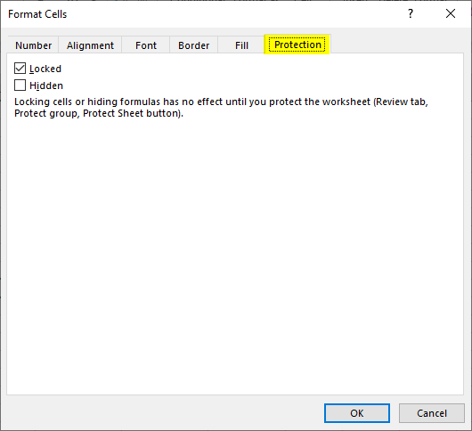
Protection
Locking Cells
This property returns True if the object is locked, False if the object can be modified when the sheet is protected, or Null if the specified range contains both locked and unlocked cells.
The following code example unlocks cells A1:B22 on Sheet1 so that they can be modified when the sheet is protected.
Worksheets("Sheet1").Range("A1:B22").Locked = False
Worksheets("Sheet1").Protect
Hiding Formulas
This property returns True if the formula will be hidden when the worksheet is protected, Null if the specified range contains some cells with FormulaHidden equal to True and some cells with FormulaHidden equal to False.
Don’t confuse this property with the Hidden property. The formula will not be hidden if the workbook is protected and the worksheet is not, but only if the worksheet is protected.
The following code example hides the formulas in cells A1 and C1 on Sheet1 when the worksheet is protected.
Worksheets("Sheet1").Range("A1:C1").FormulaHidden = TrueExcel for Microsoft 365 Excel 2021 Excel 2019 Excel 2016 Excel 2013 Excel 2010 Excel 2007 More…Less
Microsoft Office Excel has a number of features that make it easy to manage and analyze data. To take full advantage of these features, it is important that you organize and format data in a worksheet according to the following guidelines.
In this article
-
Data organization guidelines
-
Data format guidelines
Data organization guidelines
Put similar items in the same column Design the data so that all rows have similar items in the same column.
Keep a range of data separate Leave at least one blank column and one blank row between a related data range and other data on the worksheet. Excel can then more easily detect and select the range when you sort, filter, or insert automatic subtotals.
Position critical data above or below the range Avoid placing critical data to the left or right of the range because the data might be hidden when you filter the range.
Avoid blank rows and columns in a range Avoid putting blank rows and columns within a range of data. Do this to ensure that Excel can more easily detect and select the related data range.
Display all rows and columns in a range Make sure that any hidden rows or columns are displayed before you make changes to a range of data. When rows and columns in a range are not displayed, data can be deleted inadvertently. For more information, see Hide or display rows and columns.
Top of Page
Data format guidelines
Use column labels to identify data Create column labels in the first row of the range of data by applying a different format to the data. Excel can then use these labels to create reports and to find and organize data. Use a font, alignment, format, pattern, border, or capitalization style for column labels that is different from the format that you assign to the data in the range. Format the cells as text before you type the column labels. For more information, see Ways to format a worksheet.
Use cell borders to distinguish data When you want to separate labels from data, use cell borders — not blank rows or dashed lines — to insert lines below the labels. For more information, see Apply or remove cell borders on a worksheet.
Avoid leading or trailing spaces to avoid errors Avoid inserting spaces at the beginning or end of a cell to indent data. These extra spaces can affect sorting, searching, and the format that is applied to a cell. Instead of typing spaces to indent data, you can use the Increase Indent command within the cell. For more information, see Reposition the data in a cell.
Extend data formats and formulas When you add new rows of data to the end of a data range, Excel extends consistent formatting and formulas. Three of the five preceding cells must use the same format for that format to be extended. All of the preceding formulas must be consistent for a formula to be extended. For more information, see Fill data automatically in worksheet cells.
Use an Excel table format to work with related data You can turn a contiguous range of cells on your worksheet into an Excel table. Data that is defined by the table can be manipulated independently of data outside of the table, and you can use specific table features to quickly sort, filter, total, or calculate the data in the table. You can also use the table feature to compartmentalize sets of related data by organizing that data in multiple tables on a single worksheet. For more information, see Overview of Excel tables.
Top of Page
Need more help?
Want more options?
Explore subscription benefits, browse training courses, learn how to secure your device, and more.
Communities help you ask and answer questions, give feedback, and hear from experts with rich knowledge.
На чтение 18 мин. Просмотров 74.9k.

сэр Артур Конан Дойл
Это большая ошибка — теоретизировать, прежде чем кто-то получит данные
Эта статья охватывает все, что вам нужно знать об использовании ячеек и диапазонов в VBA. Вы можете прочитать его от начала до конца, так как он сложен в логическом порядке. Или использовать оглавление ниже, чтобы перейти к разделу по вашему выбору.
Рассматриваемые темы включают свойство смещения, чтение
значений между ячейками, чтение значений в массивы и форматирование ячеек.
Содержание
- Краткое руководство по диапазонам и клеткам
- Введение
- Важное замечание
- Свойство Range
- Свойство Cells рабочего листа
- Использование Cells и Range вместе
- Свойство Offset диапазона
- Использование диапазона CurrentRegion
- Использование Rows и Columns в качестве Ranges
- Использование Range вместо Worksheet
- Чтение значений из одной ячейки в другую
- Использование метода Range.Resize
- Чтение Value в переменные
- Как копировать и вставлять ячейки
- Чтение диапазона ячеек в массив
- Пройти через все клетки в диапазоне
- Форматирование ячеек
- Основные моменты
Краткое руководство по диапазонам и клеткам
| Функция | Принимает | Возвращает | Пример | Вид |
| Range | адреса ячеек |
диапазон ячеек |
.Range(«A1:A4») | $A$1:$A$4 |
| Cells | строка, столбец |
одна ячейка |
.Cells(1,5) | $E$1 |
| Offset | строка, столбец |
диапазон | .Range(«A1:A2») .Offset(1,2) |
$C$2:$C$3 |
| Rows | строка (-и) | одна или несколько строк |
.Rows(4) .Rows(«2:4») |
$4:$4 $2:$4 |
| Columns | столбец (-цы) |
один или несколько столбцов |
.Columns(4) .Columns(«B:D») |
$D:$D $B:$D |
Введение
Это третья статья, посвященная трем основным элементам VBA. Этими тремя элементами являются Workbooks, Worksheets и Ranges/Cells. Cells, безусловно, самая важная часть Excel. Почти все, что вы делаете в Excel, начинается и заканчивается ячейками.
Вы делаете три основных вещи с помощью ячеек:
- Читаете из ячейки.
- Пишите в ячейку.
- Изменяете формат ячейки.
В Excel есть несколько методов для доступа к ячейкам, таких как Range, Cells и Offset. Можно запутаться, так как эти функции делают похожие операции.
В этой статье я расскажу о каждом из них, объясню, почему они вам нужны, и когда вам следует их использовать.
Давайте начнем с самого простого метода доступа к ячейкам — с помощью свойства Range рабочего листа.
Важное замечание
Я недавно обновил эту статью, сейчас использую Value2.
Вам может быть интересно, в чем разница между Value, Value2 и значением по умолчанию:
' Value2
Range("A1").Value2 = 56

' Value
Range("A1").Value = 56

' По умолчанию используется значение
Range("A1") = 56
Использование Value может усечь число, если ячейка отформатирована, как валюта. Если вы не используете какое-либо свойство, по умолчанию используется Value.
Лучше использовать Value2, поскольку он всегда будет возвращать фактическое значение ячейки.
Свойство Range
Рабочий лист имеет свойство Range, которое можно использовать для доступа к ячейкам в VBA. Свойство Range принимает тот же аргумент, что и большинство функций Excel Worksheet, например: «А1», «А3: С6» и т.д.
В следующем примере показано, как поместить значение в ячейку с помощью свойства Range.
Sub ZapisVYacheiku()

    ' Запишите число в ячейку A1 на листе 1 этой книги
    ThisWorkbook.Worksheets("Лист1").Range("A1").Value2 = 67

    ' Напишите текст в ячейку A2 на листе 1 этой рабочей книги
    ThisWorkbook.Worksheets("Лист1").Range("A2").Value2 = "Иван Петров"

    ' Запишите дату в ячейку A3 на листе 1 этой книги
    ThisWorkbook.Worksheets("Лист1").Range("A3").Value2 = #11/21/2019#

End Sub
Как видно из кода, Range является членом Worksheets, которая, в свою очередь, является членом Workbook. Иерархия такая же, как и в Excel, поэтому должно быть легко понять. Чтобы сделать что-то с Range, вы должны сначала указать рабочую книгу и рабочий лист, которому она принадлежит.
В оставшейся части этой статьи я буду использовать кодовое имя для ссылки на лист.

Следующий код показывает приведенный выше пример с использованием кодового имени рабочего листа, т.е. Лист1 вместо ThisWorkbook.Worksheets («Лист1»).
Sub IspKodImya ()

    ' Запишите число в ячейку A1 на листе 1 этой книги
     Sheet1.Range("A1").Value2 = 67

    ' Напишите текст в ячейку A2 на листе 1 этой рабочей книги
    Sheet1.Range("A2").Value2 = "Иван Петров"

    ' Запишите дату в ячейку A3 на листе 1 этой книги
    Sheet1.Range("A3").Value2 = #11/21/2019#

End Sub
Вы также можете писать в несколько ячеек, используя свойство
Range
Sub ZapisNeskol()

    ' Запишите число в диапазон ячеек
    Sheet1.Range("A1:A10").Value2 = 67

    ' Написать текст в несколько диапазонов ячеек
    Sheet1.Range("B2:B5,B7:B9").Value2 = "Иван Петров"

End Sub
Свойство Cells рабочего листа
У Объекта листа есть другое свойство, называемое Cells, которое очень похоже на Range . Есть два отличия:
- Cells возвращают диапазон только одной ячейки.
- Cells принимает строку и столбец в качестве аргументов.
В приведенном ниже примере показано, как записывать значения
в ячейки, используя свойства Range и Cells.
Sub IspCells()

    ' Написать в А1
    Sheet1.Range("A1").Value2 = 10
    Sheet1.Cells(1, 1).Value2  = 10

    ' Написать в А10
    Sheet1.Range("A10").Value2 = 10
    Sheet1.Cells(10, 1).Value2  = 10

    ' Написать в E1
    Sheet1.Range("E1").Value2 = 10
    Sheet1.Cells(1, 5).Value2  = 10

End Sub
Вам должно быть интересно, когда использовать Cells, а когда Range. Использование Range полезно для доступа к одним и тем же ячейкам при каждом запуске макроса.
Например, если вы использовали макрос для вычисления суммы и
каждый раз записывали ее в ячейку A10, тогда Range подойдет для этой задачи.
Использование свойства Cells полезно, если вы обращаетесь к
ячейке по номеру, который может отличаться. Проще объяснить это на примере.
В следующем коде мы просим пользователя указать номер столбца. Использование Cells дает нам возможность использовать переменное число для столбца.
Sub ZapisVPervuyuPustuyuYacheiku()

    Dim UserCol As Integer

    ' Получить номер столбца от пользователя
    UserCol = Application.InputBox("Пожалуйста, введите номер столбца...", Type:=1)

    ' Написать текст в выбранный пользователем столбец
    Sheet1.Cells(1, UserCol).Value2 = "Иван Петров"

End Sub
В приведенном выше примере мы используем номер для столбца,
а не букву.
Чтобы использовать Range здесь, потребуется преобразовать эти значения в ссылку на
буквенно-цифровую ячейку, например, «С1». Использование свойства Cells позволяет нам
предоставить строку и номер столбца для доступа к ячейке.
Иногда вам может понадобиться вернуть более одной ячейки, используя номера строк и столбцов. В следующем разделе показано, как это сделать.
Использование Cells и Range вместе
Как вы уже видели, вы можете получить доступ только к одной ячейке, используя свойство Cells. Если вы хотите вернуть диапазон ячеек, вы можете использовать Cells с Range следующим образом:
Sub IspCellsSRange()

    With Sheet1
        ' Запишите 5 в диапазон A1: A10, используя свойство Cells
        .Range(.Cells(1, 1), .Cells(10, 1)).Value2 = 5

        ' Диапазон B1: Z1 будет выделен жирным шрифтом
        .Range(.Cells(1, 2), .Cells(1, 26)).Font.Bold = True

    End With

End Sub
Как видите, вы предоставляете начальную и конечную ячейку
диапазона. Иногда бывает сложно увидеть, с каким диапазоном вы имеете дело,
когда значением являются все числа. Range имеет свойство Address, которое
отображает буквенно-цифровую ячейку для любого диапазона. Это может
пригодиться, когда вы впервые отлаживаете или пишете код.
В следующем примере мы распечатываем адрес используемых нами
диапазонов.
Sub PokazatAdresDiapazona()

    ' Примечание. Использование подчеркивания позволяет разделить строки кода.
    With Sheet1

        ' Запишите 5 в диапазон A1: A10, используя свойство Cells
        .Range(.Cells(1, 1), .Cells(10, 1)).Value2 = 5
        Debug.Print "Первый адрес: " _
            + .Range(.Cells(1, 1), .Cells(10, 1)).Address

        ' Диапазон B1: Z1 будет выделен жирным шрифтом
        .Range(.Cells(1, 2), .Cells(1, 26)).Font.Bold = True
        Debug.Print "Второй адрес : " _
            + .Range(.Cells(1, 2), .Cells(1, 26)).Address

    End With

End Sub
В примере я использовал Debug.Print для печати в Immediate Window. Для просмотра этого окна выберите «View» -> «в Immediate Window» (Ctrl + G).


Свойство Offset диапазона
У диапазона есть свойство, которое называется Offset. Термин «Offset» относится к отсчету от исходной позиции. Он часто используется в определенных областях программирования. С помощью свойства «Offset» вы можете получить диапазон ячеек того же размера и на определенном расстоянии от текущего диапазона. Это полезно, потому что иногда вы можете выбрать диапазон на основе определенного условия. Например, на скриншоте ниже есть столбец для каждого дня недели. Учитывая номер дня (т.е. понедельник = 1, вторник = 2 и т.д.). Нам нужно записать значение в правильный столбец.

Сначала мы попытаемся сделать это без использования Offset.
' Это Sub тесты с разными значениями
Sub TestSelect()

    ' Понедельник
    SetValueSelect 1, 111.21
    ' Среда
    SetValueSelect 3, 456.99
    ' Пятница
    SetValueSelect 5, 432.25
    ' Воскресение
    SetValueSelect 7, 710.17

End Sub

' Записывает значение в столбец на основе дня
Public Sub SetValueSelect(lDay As Long, lValue As Currency)

    Select Case lDay
        Case 1: Sheet1.Range("H3").Value2 = lValue
        Case 2: Sheet1.Range("I3").Value2 = lValue
        Case 3: Sheet1.Range("J3").Value2 = lValue
        Case 4: Sheet1.Range("K3").Value2 = lValue
        Case 5: Sheet1.Range("L3").Value2 = lValue
        Case 6: Sheet1.Range("M3").Value2 = lValue
        Case 7: Sheet1.Range("N3").Value2 = lValue
    End Select

End Sub
Как видно из примера, нам нужно добавить строку для каждого возможного варианта. Это не идеальная ситуация. Использование свойства Offset обеспечивает более чистое решение.
' Это Sub тесты с разными значениями
Sub TestOffset()

    DayOffSet 1, 111.01
    DayOffSet 3, 456.99
    DayOffSet 5, 432.25
    DayOffSet 7, 710.17

End Sub

Public Sub DayOffSet(lDay As Long, lValue As Currency)

    ' Мы используем значение дня с Offset, чтобы указать правильный столбец
    Sheet1.Range("G3").Offset(, lDay).Value2 = lValue

End Sub
Как видите, это решение намного лучше. Если количество дней увеличилось, нам больше не нужно добавлять код. Чтобы Offset был полезен, должна быть какая-то связь между позициями ячеек. Если столбцы Day в приведенном выше примере были случайными, мы не могли бы использовать Offset. Мы должны были бы использовать первое решение.
Следует иметь в виду, что Offset сохраняет размер диапазона. Итак .Range («A1:A3»).Offset (1,1) возвращает диапазон B2:B4. Ниже приведены еще несколько примеров использования Offset.
Sub IspOffset()

    ' Запись в В2 - без Offset
    Sheet1.Range("B2").Offset().Value2 = "Ячейка B2"

    ' Написать в C2 - 1 столбец справа
    Sheet1.Range("B2").Offset(, 1).Value2 = "Ячейка C2"

    ' Написать в B3 - 1 строка вниз
    Sheet1.Range("B2").Offset(1).Value2 = "Ячейка B3"

    ' Запись в C3 - 1 столбец справа и 1 строка вниз
    Sheet1.Range("B2").Offset(1, 1).Value2 = "Ячейка C3"

    ' Написать в A1 - 1 столбец слева и 1 строка вверх
    Sheet1.Range("B2").Offset(-1, -1).Value2 = "Ячейка A1"

    ' Запись в диапазон E3: G13 - 1 столбец справа и 1 строка вниз
    Sheet1.Range("D2:F12").Offset(1, 1).Value2 = "Ячейки E3:G13"

End Sub
Использование диапазона CurrentRegion
CurrentRegion возвращает диапазон всех соседних ячеек в данный диапазон. На скриншоте ниже вы можете увидеть два CurrentRegion. Я добавил границы, чтобы прояснить CurrentRegion.

Строка или столбец пустых ячеек означает конец CurrentRegion.
Вы можете вручную проверить
CurrentRegion в Excel, выбрав диапазон и нажав Ctrl + Shift + *.
Если мы возьмем любой диапазон
ячеек в пределах границы и применим CurrentRegion, мы вернем диапазон ячеек во
всей области.
Например:
Range («B3»). CurrentRegion вернет диапазон B3:D14
Range («D14»). CurrentRegion вернет диапазон B3:D14
Range («C8:C9»). CurrentRegion вернет диапазон B3:D14 и так далее
Как пользоваться
Мы получаем CurrentRegion следующим образом
' CurrentRegion вернет B3:D14 из приведенного выше примера
Dim rg As Range
Set rg = Sheet1.Range("B3").CurrentRegion
Только чтение строк данных
Прочитать диапазон из второй строки, т.е. пропустить строку заголовка.
' CurrentRegion вернет B3:D14 из приведенного выше примера
Dim rg As Range
Set rg = Sheet1.Range("B3").CurrentRegion

' Начало в строке 2 - строка после заголовка
Dim i As Long
For i = 2 To rg.Rows.Count
    ' текущая строка, столбец 1 диапазона
    Debug.Print rg.Cells(i, 1).Value2
Next i
Удалить заголовок
Удалить строку заголовка (т.е. первую строку) из диапазона. Например, если диапазон — A1:D4, это возвратит A2:D4
' CurrentRegion вернет B3:D14 из приведенного выше примера
Dim rg As Range
Set rg = Sheet1.Range("B3").CurrentRegion

' Удалить заголовок
Set rg = rg.Resize(rg.Rows.Count - 1).Offset(1)

' Начните со строки 1, так как нет строки заголовка
Dim i As Long
For i = 1 To rg.Rows.Count
    ' текущая строка, столбец 1 диапазона
    Debug.Print rg.Cells(i, 1).Value2
Next i
Использование Rows и Columns в качестве Ranges
Если вы хотите что-то сделать со всей строкой или столбцом,
вы можете использовать свойство «Rows и
Columns» на рабочем листе. Они оба принимают один параметр — номер строки
или столбца, к которому вы хотите получить доступ.
Sub IspRowIColumns()

    ' Установите размер шрифта столбца B на 9
    Sheet1.Columns(2).Font.Size = 9

    ' Установите ширину столбцов от D до F
    Sheet1.Columns("D:F").ColumnWidth = 4

    ' Установите размер шрифта строки 5 до 18
    Sheet1.Rows(5).Font.Size = 18

End Sub
Использование Range вместо Worksheet
Вы также можете использовать Cella, Rows и Columns, как часть Range, а не как часть Worksheet. У вас может быть особая необходимость в этом, но в противном случае я бы избегал практики. Это делает код более сложным. Простой код — твой друг. Это уменьшает вероятность ошибок.
Код ниже выделит второй столбец диапазона полужирным. Поскольку диапазон имеет только две строки, весь столбец считается B1:B2
Sub IspColumnsVRange()

    ' Это выделит B1 и B2 жирным шрифтом.
    Sheet1.Range("A1:C2").Columns(2).Font.Bold = True

End Sub
Чтение значений из одной ячейки в другую
В большинстве примеров мы записали значения в ячейку. Мы
делаем это, помещая диапазон слева от знака равенства и значение для размещения
в ячейке справа. Для записи данных из одной ячейки в другую мы делаем то же
самое. Диапазон назначения идет слева, а диапазон источника — справа.
В следующем примере показано, как это сделать:
Sub ChitatZnacheniya()

    ' Поместите значение из B1 в A1
    Sheet1.Range("A1").Value2 = Sheet1.Range("B1").Value2

    ' Поместите значение из B3 в лист2 в ячейку A1
    Sheet1.Range("A1").Value2 = Sheet2.Range("B3").Value2

    ' Поместите значение от B1 в ячейки A1 до A5
    Sheet1.Range("A1:A5").Value2 = Sheet1.Range("B1").Value2

    ' Вам необходимо использовать свойство «Value», чтобы прочитать несколько ячеек
    Sheet1.Range("A1:A5").Value2 = Sheet1.Range("B1:B5").Value2

End Sub
Как видно из этого примера, невозможно читать из нескольких ячеек. Если вы хотите сделать это, вы можете использовать функцию копирования Range с параметром Destination.
Sub KopirovatZnacheniya()

    ' Сохранить диапазон копирования в переменной
    Dim rgCopy As Range
    Set rgCopy = Sheet1.Range("B1:B5")

    ' Используйте это для копирования из более чем одной ячейки
    rgCopy.Copy Destination:=Sheet1.Range("A1:A5")

    ' Вы можете вставить в несколько мест назначения
    rgCopy.Copy Destination:=Sheet1.Range("A1:A5,C2:C6")

End Sub
Функция Copy копирует все, включая формат ячеек. Это тот же результат, что и ручное копирование и вставка выделения. Подробнее об этом вы можете узнать в разделе «Копирование и вставка ячеек»
Использование метода Range.Resize
При копировании из одного диапазона в другой с использованием присваивания (т.е. знака равенства) диапазон назначения должен быть того же размера, что и исходный диапазон.
Использование функции Resize позволяет изменить размер
диапазона до заданного количества строк и столбцов.
Например:
Sub ResizePrimeri()

    ' Печатает А1
    Debug.Print Sheet1.Range("A1").Address

    ' Печатает A1:A2
    Debug.Print Sheet1.Range("A1").Resize(2, 1).Address

    ' Печатает A1:A5
    Debug.Print Sheet1.Range("A1").Resize(5, 1).Address

    ' Печатает A1:D1
    Debug.Print Sheet1.Range("A1").Resize(1, 4).Address

    ' Печатает A1:C3
    Debug.Print Sheet1.Range("A1").Resize(3, 3).Address

End Sub
Когда мы хотим изменить наш целевой диапазон, мы можем
просто использовать исходный размер диапазона.
Другими словами, мы используем количество строк и столбцов
исходного диапазона в качестве параметров для изменения размера:
Sub Resize()

    Dim rgSrc As Range, rgDest As Range

    ' Получить все данные в текущей области
    Set rgSrc = Sheet1.Range("A1").CurrentRegion

      ' Получить диапазон назначения
    Set rgDest = Sheet2.Range("A1")
    Set rgDest = rgDest.Resize(rgSrc.Rows.Count, rgSrc.Columns.Count)

    rgDest.Value2 = rgSrc.Value2

End Sub
Мы можем сделать изменение размера в одну строку, если нужно:
Sub Resize2()

    Dim rgSrc As Range

    ' Получить все данные в ткущей области
    Set rgSrc = Sheet1.Range("A1").CurrentRegion

    With rgSrc
        Sheet2.Range("A1").Resize(.Rows.Count, .Columns.Count) = .Value2
    End With

End Sub
Чтение Value в переменные
Мы рассмотрели, как читать из одной клетки в другую. Вы также можете читать из ячейки в переменную. Переменная используется для хранения значений во время работы макроса. Обычно вы делаете это, когда хотите манипулировать данными перед тем, как их записать. Ниже приведен простой пример использования переменной. Как видите, значение элемента справа от равенства записывается в элементе слева от равенства.
Sub IspVar()

    ' Создайте
    Dim val As Integer

    ' Читать число из ячейки
    val = Sheet1.Range("A1").Value2

    ' Добавить 1 к значению
    val = val + 1

    ' Запишите новое значение в ячейку
    Sheet1.Range("A2").Value2 = val

End Sub
Для чтения текста в переменную вы используете переменную
типа String.
Sub IspVarText()

    ' Объявите переменную типа string
    Dim sText As String

    ' Считать значение из ячейки
    sText = Sheet1.Range("A1").Value2

    ' Записать значение в ячейку
    Sheet1.Range("A2").Value2 = sText

End Sub
Вы можете записать переменную в диапазон ячеек. Вы просто
указываете диапазон слева, и значение будет записано во все ячейки диапазона.
Sub VarNeskol()

    ' Считать значение из ячейки
    Sheet1.Range("A1:B10").Value2 = 66

End Sub
Вы не можете читать из нескольких ячеек в переменную. Однако
вы можете читать массив, который представляет собой набор переменных. Мы
рассмотрим это в следующем разделе.
Как копировать и вставлять ячейки
Если вы хотите скопировать и вставить диапазон ячеек, вам не
нужно выбирать их. Это распространенная ошибка, допущенная новыми пользователями
VBA.
Вы можете просто скопировать ряд ячеек, как здесь:
Range("A1:B4").Copy Destination:=Range("C5")
При использовании этого метода копируется все — значения,
форматы, формулы и так далее. Если вы хотите скопировать отдельные элементы, вы
можете использовать свойство PasteSpecial
диапазона.
Работает так:
Range("A1:B4").Copy
Range("F3").PasteSpecial Paste:=xlPasteValues
Range("F3").PasteSpecial Paste:=xlPasteFormats
Range("F3").PasteSpecial Paste:=xlPasteFormulas
В следующей таблице приведен полный список всех типов вставок.
| Виды вставок |
| xlPasteAll |
| xlPasteAllExceptBorders |
| xlPasteAllMergingConditionalFormats |
| xlPasteAllUsingSourceTheme |
| xlPasteColumnWidths |
| xlPasteComments |
| xlPasteFormats |
| xlPasteFormulas |
| xlPasteFormulasAndNumberFormats |
| xlPasteValidation |
| xlPasteValues |
| xlPasteValuesAndNumberFormats |
Чтение диапазона ячеек в массив
Вы также можете скопировать значения, присвоив значение
одного диапазона другому.
Range("A3:Z3").Value2 = Range("A1:Z1").Value2
Значение диапазона в этом примере считается вариантом массива. Это означает, что вы можете легко читать из диапазона ячеек в массив. Вы также можете писать из массива в диапазон ячеек. Если вы не знакомы с массивами, вы можете проверить их в этой статье.
В следующем коде показан пример использования массива с
диапазоном.
Sub ChitatMassiv()

    ' Создать динамический массив
    Dim StudentMarks() As Variant

    ' Считать 26 значений в массив из первой строки
    StudentMarks = Range("A1:Z1").Value2

    ' Сделайте что-нибудь с массивом здесь

    ' Запишите 26 значений в третью строку
    Range("A3:Z3").Value2 = StudentMarks

End Sub
Имейте в виду, что массив, созданный для чтения, является
двумерным массивом. Это связано с тем, что электронная таблица хранит значения
в двух измерениях, то есть в строках и столбцах.
Пройти через все клетки в диапазоне
Иногда вам нужно просмотреть каждую ячейку, чтобы проверить значение.
Вы можете сделать это, используя цикл For Each, показанный в следующем коде.
Sub PeremeschatsyaPoYacheikam()

    ' Пройдите через каждую ячейку в диапазоне
    Dim rg As Range
    For Each rg In Sheet1.Range("A1:A10,A20")
        ' Распечатать адрес ячеек, которые являются отрицательными
        If rg.Value < 0 Then
            Debug.Print rg.Address + " Отрицательно."
        End If
    Next

End Sub
Вы также можете проходить последовательные ячейки, используя
свойство Cells и стандартный цикл For.
Стандартный цикл более гибок в отношении используемого вами
порядка, но он медленнее, чем цикл For Each.
Sub PerehodPoYacheikam()

    ' Пройдите клетки от А1 до А10
    Dim i As Long
    For i = 1 To 10
        ' Распечатать адрес ячеек, которые являются отрицательными
        If Range("A" & i).Value < 0 Then
            Debug.Print Range("A" & i).Address + " Отрицательно."
        End If
    Next

    ' Пройдите в обратном порядке, то есть от A10 до A1
    For i = 10 To 1 Step -1
        ' Распечатать адрес ячеек, которые являются отрицательными
        If Range("A" & i) < 0 Then
            Debug.Print Range("A" & i).Address + " Отрицательно."
        End If
    Next

End Sub
Форматирование ячеек
Иногда вам нужно будет отформатировать ячейки в электронной
таблице. Это на самом деле очень просто. В следующем примере показаны различные
форматы, которые можно добавить в любой диапазон ячеек.
Sub FormatirovanieYacheek()

    With Sheet1

        ' Форматировать шрифт
        .Range("A1").Font.Bold = True
        .Range("A1").Font.Underline = True
        .Range("A1").Font.Color = rgbNavy

        ' Установите числовой формат до 2 десятичных знаков
        .Range("B2").NumberFormat = "0.00"
        ' Установите числовой формат даты
        .Range("C2").NumberFormat = "dd/mm/yyyy"
        ' Установите формат чисел на общий
        .Range("C3").NumberFormat = "Общий"
        ' Установить числовой формат текста
        .Range("C4").NumberFormat = "Текст"

        ' Установите цвет заливки ячейки
        .Range("B3").Interior.Color = rgbSandyBrown

        ' Форматировать границы
        .Range("B4").Borders.LineStyle = xlDash
        .Range("B4").Borders.Color = rgbBlueViolet

    End With

End Sub
Основные моменты
Ниже приводится краткое изложение основных моментов
- Range возвращает диапазон ячеек
- Cells возвращают только одну клетку
- Вы можете читать из одной ячейки в другую
- Вы можете читать из диапазона ячеек в другой диапазон ячеек.
- Вы можете читать значения из ячеек в переменные и наоборот.
- Вы можете читать значения из диапазонов в массивы и наоборот
- Вы можете использовать цикл For Each или For, чтобы проходить через каждую ячейку в диапазоне.
- Свойства Rows и Columns позволяют вам получить доступ к диапазону ячеек этих типов

In Microsoft Excel, a range is a collection of cells. A range can be 2 or more cells and those cells don’t necessarily have to be adjacent to each other. Let’s look at some examples to quickly demonstrate the different types of ranges.
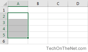
Vertical Range
This vertical range is A2:A5. In this example, if you had selected the entire column A, the range would be A:A.
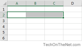
Horizontal Range
This horizontal range is A2:C2. In this example, if you selected the entire row 2, the range would have be 2:2.
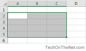
Mixed Range
This mixed range is A2:C5. This is a collection of cells that can be from multiple rows and columns.
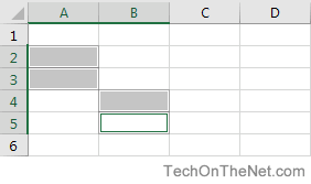
Multiple Selection Range
This multiple selection range is A2:A3,B4:B5. This is a collection of cells that does not have to be adjacent.
Each range has its own set of coordinates or position in the worksheet such as A2:A5, A2:C2, A2:C5, and so on.
There are many things that you can do with ranges in Excel such as copying, moving, formatting, and naming ranges. Here is a list of topics that explain how to use ranges in Excel.
This tutorial about cell format types in Excel is an essential part of your learning of Excel and will definitely do a lot of good to you in your future use of this software, as a lot of tasks in Excel sheets are based on cells format, as well as several errors are due to a bad implementation of it.
A good comprehension of the cell format types will build your knowledge on a solid basis to master Excel basics and will considerably save you time and effort when any related issue occurs.
A- Introduction
Excel software formats the cells depending on what type of information they contain.
To update the format of the highlighted cell, go to the “Home” tab of the ribbon and click, in the “Number” group of commands on the “Number Format” drop-down list.
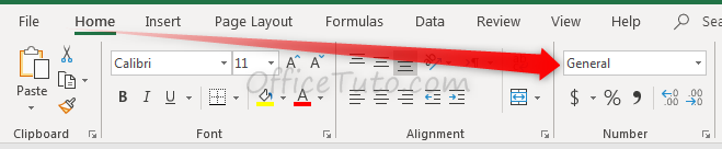
The drop-down list allows the selection to be changed.
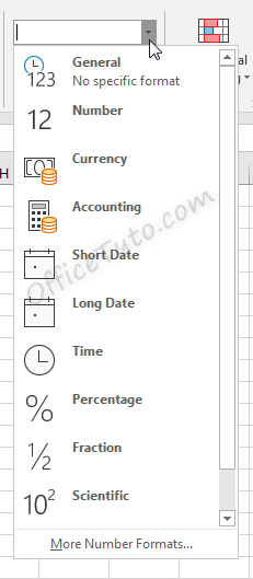
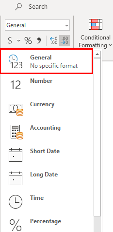
Cell formatting options in the “Number Format” drop-down list are:
- General
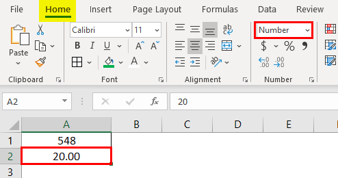
- Number
- Currency
- Accounting
- Short Date
- Long Date
- Time
- Percentage
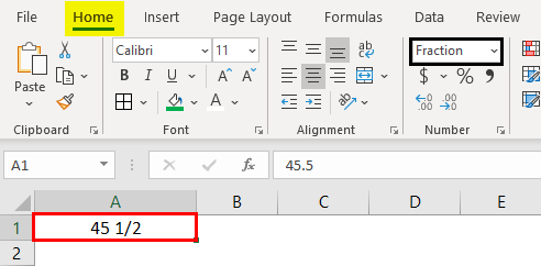
- Fraction
- Scientific
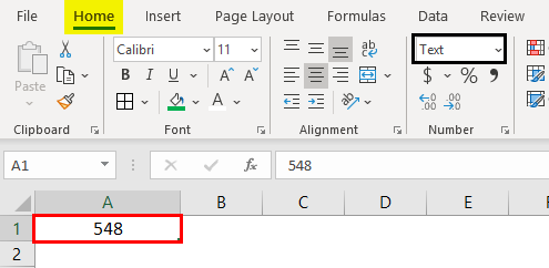
- Text
- And the “More Number Formats” option.
Clicking the “More Number Formats” option brings up additional options for formatting cells, including the ability to do special and custom formatting options.
These options are discussed in detail in the below sections.
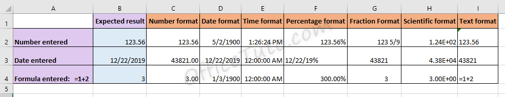
Cell format types in Excel are: General, Number, Currency, Accounting, Date, Time, Percentage, Fraction, Scientific, Text, Special (Zip Code, Zip Code + 4, Phone Number, Social Security Number), and Custom. You can get them from the “Number Format” drop-down list in the “Home” tab, or from the launcher arrow below it.
I will detail each one of them in the following sections:
1- General format
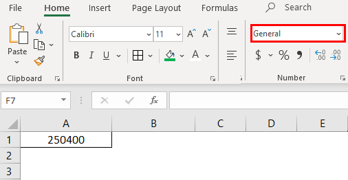
By default, cells are formatted as “General”, which could store any type of information. The General format means that no specific format is applied to the selected cell.
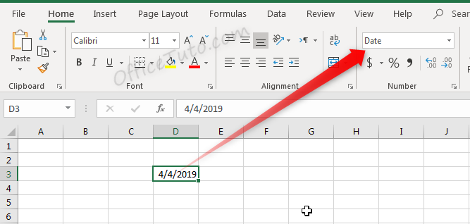
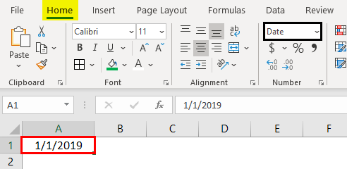
When information is typed into a cell, the cell format may change automatically. For example, if I enter “4/4/19” into a cell and press enter, then highlight the cell to view details about it, the cell format will be listed as “Date” instead of “General”.
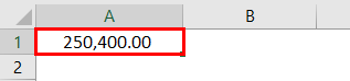
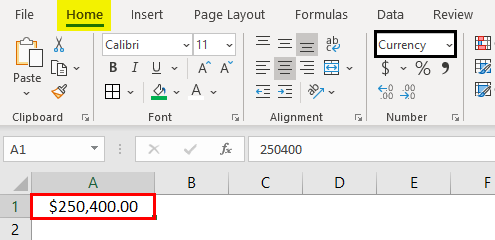
Similarly, we can update a cell’s format before or after entering data to adjust the way the data appears. Changing the format of a cell to “Currency” will make it so information entered is displayed as a dollar amount.
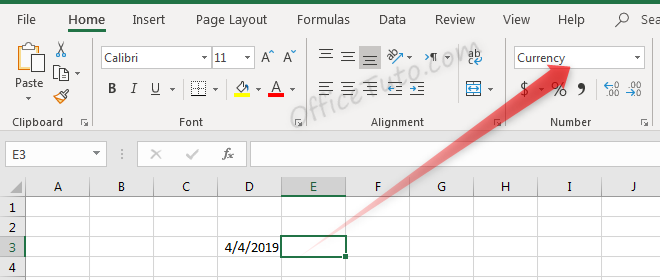
Typing a number into this cell and pressing enter will not just show that number, but will instead format it accordingly.
Before pressing enter, Excel shows the value which was typed: “4”.
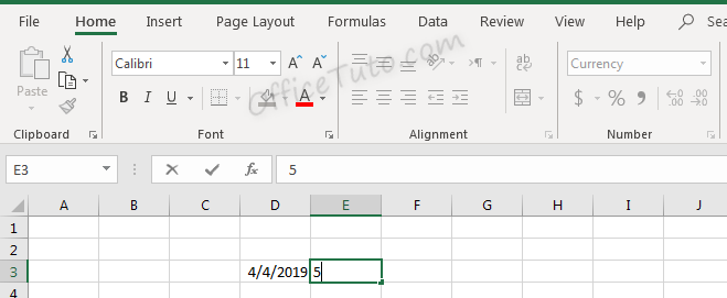
After pressing enter, the value is updated based on the formatting type selected.
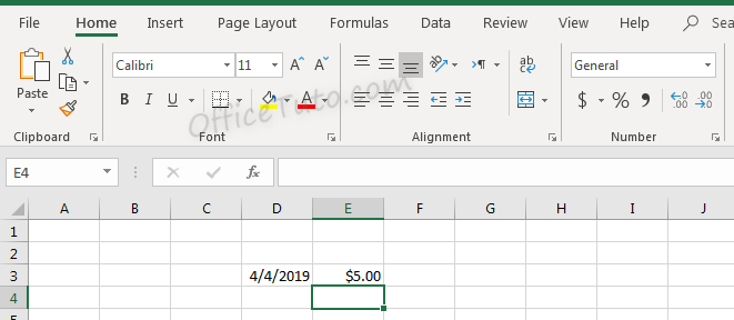
Don’t let the format type showed in the illustration at the drop-down list confusing you; it is reflecting the cell below (i.e. E4), since we validated by an Enter.
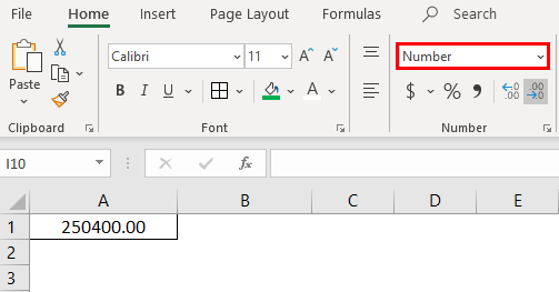
2- Number format
Cells formatted as numbers behave differently than general formatted cells. By default, when a number is entered, or when a cell is formatted as a number already, the alignment of the information within the cell will be on the right instead of on the left. This makes it easier to read a list of numbers such as the below.
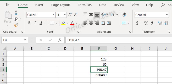
Note in the above screenshot that since we didn’t choose the “Number” format for our cells, they still have a “General” one. They are numbers for Excel (meaning, we can do calculations on them), but they didn’t have yet the number format and its formatting aspects:
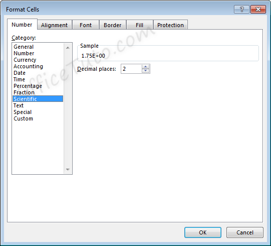
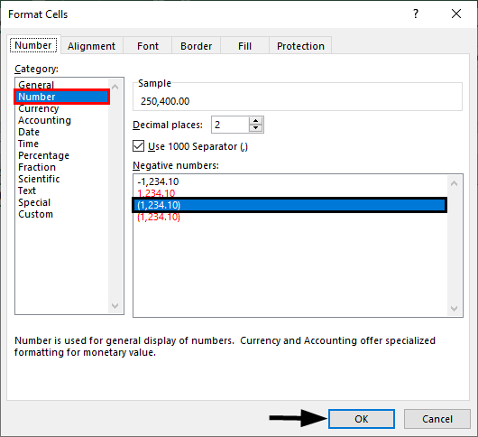
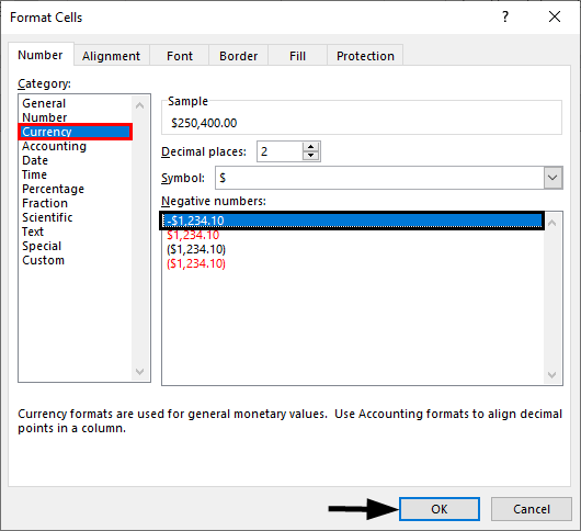
You can set the formatting options for Excel numbers in the “Format Cells” dialog box.
To do that, select the cell or the range of cells you want to set the formatting options for their numbers, and go to the “Home” tab of the ribbon, then in the “Number” group of commands, click on the launcher of the dialog box (the arrow on the right-down side of the group).
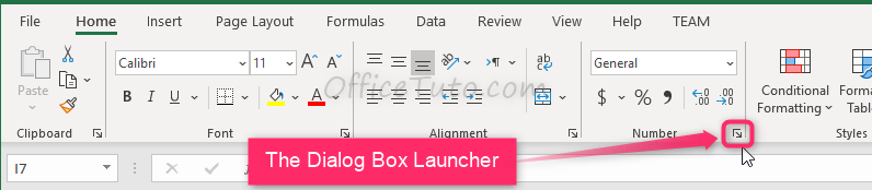
Excel opens the “Format Cells” dialog box in its “Number” tab. Click in the “Category” pane on “Number”.
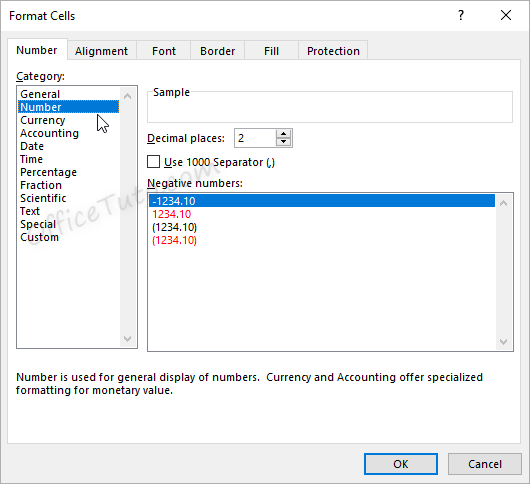
- In this dialog box, you can decide how many decimal places to display by updating options in the “Decimal places” field.
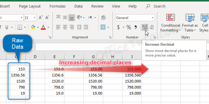
Note that this feature is also available in the “Home” tab of the ribbon where you can go to the “Number” group of commands and click the Increase Decimal ![]() or Decrease Decimal
or Decrease Decimal ![]() buttons.
buttons.
Here is the result of consecutive increasing of decimal places on our example of data (1 decimal; 2 decimals; and 3 decimals):
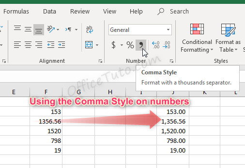
- You can also decide if commas should be shown in the display as a thousand separator, by updating the “Use 1000 Separator (,)” option in the “Format Cells” dialog box.
This feature is also available in the “Home” tab of the ribbon by clicking the “Comma Style” button ![]() in the “Number” group of commands.
in the “Number” group of commands.
Note that using the Comma Style button will automatically set the format to Accounting.
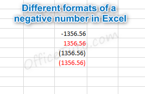
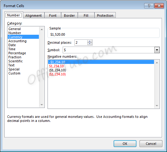
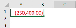
- Another option from the Format Cells dialog box is to decide how negative numbers should display by using the “Negative numbers” field.
There are four options for displaying negative
numbers.
- Display
negative numbers with a negative sign before the number. - Display
negative numbers in red. - Display
negative numbers in parentheses. - Display
negative numbers in red and in parentheses.
3- Currency format
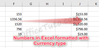
Cells formatted as currency have a currency symbol such as a dollar sign $ immediately to the left of the number in the cell, and contain two numbers after the decimal by default.
The alignment of numbers in currency formatted cells will be on the right for readability.
Currency formatting options are similar to
number formatting options, apart from the currency symbol display.
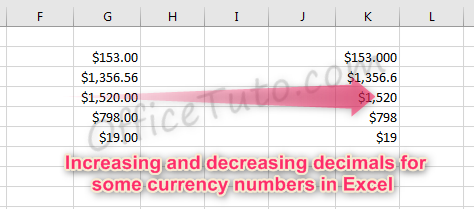
- As with regular number formatting, you can decide, in the “Format Cells” dialog box, how many decimal places to display by updating the field “Decimal places”.
You can also find this feature in the “Home” tab of the ribbon, by going to the “Number” group of commands and clicking the Increase Decimal ![]() or Decrease Decimal
or Decrease Decimal ![]() .
.
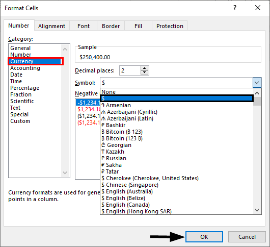
- You can also decide what currency symbol should be shown in the display by updating the “Symbol” field in the “Format Cells” dialog box.
- As with regular number formatting, you can also decide how negative numbers should display by updating the “Negative numbers” field in the “Format Cells” dialog box.
There are four
options for displaying negative numbers.
- Display
negative numbers with a negative sign before the number. - Display
negative numbers in red. - Display
negative numbers in parentheses. - Display
negative numbers in red and in parentheses.
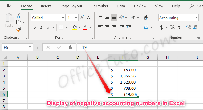
4- Accounting format
Like with the currency format, cells formatted as accounting have a currency symbol such as a dollar sign $; however, this symbol is to the far left of the cell, while the alignment of numbers in the cell is on the right. Accounting numbers contain two numbers after the decimal by default.
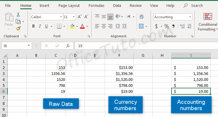
Clicking the “Accounting Number Format” button ![]() in the “Number” group of commands of the “Home” tab, will quickly format a cell or cells as Accounting.
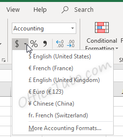
in the “Number” group of commands of the “Home” tab, will quickly format a cell or cells as Accounting.
The down arrow to the right of the Accounting Number Format button allows selection between common symbols used for accounting, including English (dollar sign), English (pound), Euro, Chinese, and French symbols.
Accounting formatting options in the “Format Cells” dialog box (“Home” tab of the ribbon, in the “Number” group of commands, click on the launcher of the “Number Format” dialog box), are similar to number and currency formatting options.
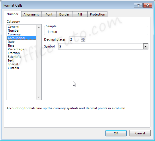
- You can decide how many decimal places to display by updating its option in the “Format Cells” dialog box.
As mentioned before in this tutorial, this feature is also available directly in the “Home” tab of the ribbon by clicking the Increase Decimal ![]() or Decrease Decimal
or Decrease Decimal ![]() buttons in the “Number” group of commands.
buttons in the “Number” group of commands.
- You can also decide in the “Format Cells” dialog box, what currency symbol should be shown in the display by using the “Symbol” drop-down list.
This dropdown gives a much broader list of options than the “Accounting Number Format” option in the “Home” tab of the ribbon.
Note that with the Accounting formatting option, negative numbers display in parentheses by default. There are not options to change this.
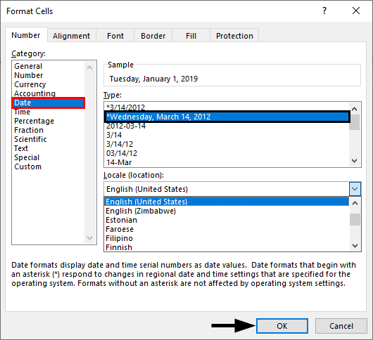
5- Date format
There are options for “Short Date” and “Long Date” in the “Number Format” dropdown list of the “Home” tab.
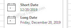
Short date shows the date with slashes separating month, day, and year. The order of the month and day may vary depending on your computer’s location settings.
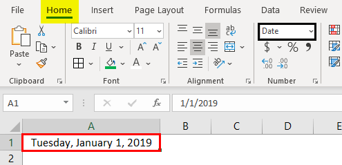
Long date shows the date with the day of the week, month, day, and year separated by commas.
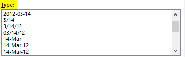
More options for formatting dates are available in the “Format Cells” dialog box (accessible by clicking in the “Number Format” dropdown list of the “Home” tab and choosing the “More Number Formats” option at the bottom).
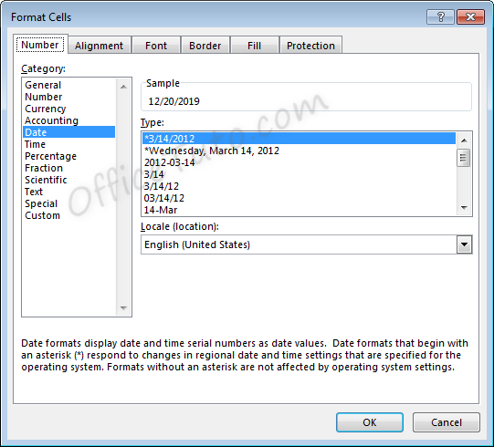
- You can choose from a long list of available date formats.
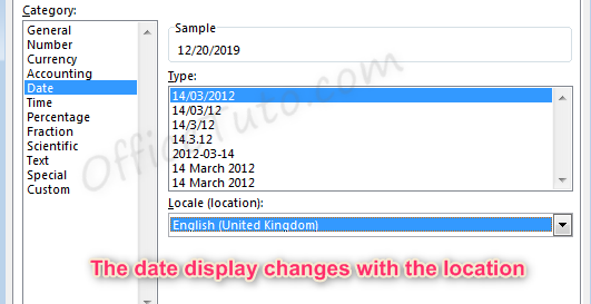
- You can update the location settings used for formatting the date. This will alter the list of format options in the above list and will adjust the display and potentially the order of the elements (day, month, year) within the date.
Note the below example when we switch from English (United States) format to English (United Kingdom) format.
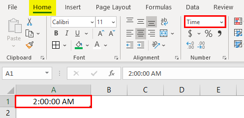
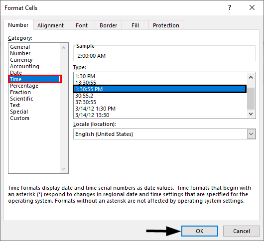
6- Time format
Cells formatted as time display the time of
day. The default time display is based on your computer’s location settings.
Time formatting options are available in the “Format Cells” dialog box (accessible by choosing the “More Number Formats” option at the bottom of the “Number Format” dropdown list in the “Home” tab of the ribbon).
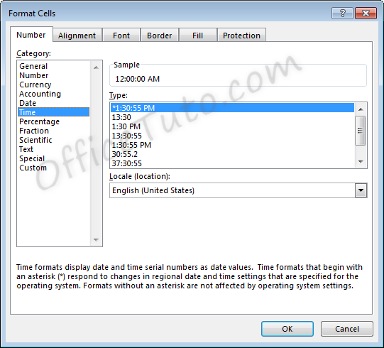
- You can choose from a long list of available time formats.
- You can update the location settings used for formatting the time. This will alter the list of format options in the above list and will adjust the display.
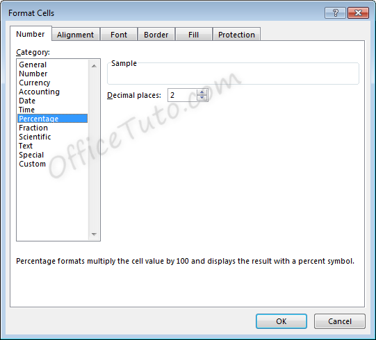
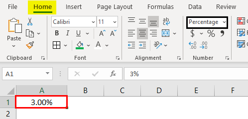
7- Percentage format
Cells formatted as percentage display a percent sign to the right of the number. You can change the format of a cell to a percentage using the “Number Format” dropdown list, or by clicking the “Percent Style” button ![]() . Both options are accessible from the “Home” tab of the ribbon, in the “Number” group of commands.
. Both options are accessible from the “Home” tab of the ribbon, in the “Number” group of commands.
Note that updating a number to a percentage
will expect that the number already contains the decimal. For example:
A cell containing the value 0.08, as a percentage, will show 8%.
A cell containing the value 8, as a percentage, will show 800%.
Percentage formatting options are available in the “Format Cells” dialog box, accessible by clicking on “More Number Formats” of the “Number Format” dropdown list in the “Home” tab of the ribbon.
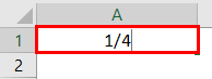
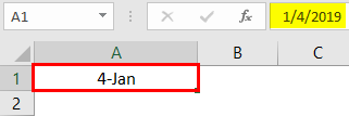
8- Fraction format
Cells formatted as a fraction display with a slash
symbol separating the numerator and denominator.
Fraction formatting options are available in the “Format Cells” dialog box, accessible by clicking in the “Home” tab of the ribbon, on “More Number Formats” of the “Number Format” dropdown list.
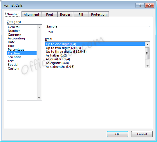
- Note that
when selecting the format to use for a fraction, Excel will round to the
nearest fraction where the formatting criteria can be met.
As an example, if the
formatting option selected is “Up to one digit”, entering a fraction with two
digits will cause rounding to occur. For example, with the setting of “Up to
one digit”,
If we enter a value of 7/16, the value displayed will be 4/9, as converting to 9ths was the option with only one digit which required the least amount of rounding.
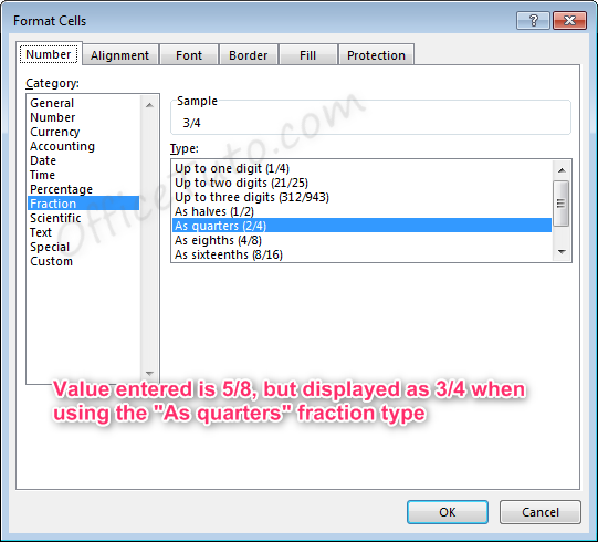
For another example, if the formatting option selected is “As quarters”, entering a fraction that cannot be expressed in quarters (divisible by four) will also cause rounding to occur.
If we enter a value of 5/8, the value displayed will be 3/4. Excel rounded up to 6/8, or 3/4, which was the closest option divisible by four.
- Also note
that for the formatting options with “Up to x digits”, Excel will always round
down to the lowest exact equivalent fraction when possible.
For example, if we enter a value of 2/4 with one of these formatting options active, the value displayed will be 1/2, as this is the mathematical equivalent. This behavior will not take place for formatting options “As…”, since these specifically determine what the denominator should be.
- Fractions listed as more than a whole (meaning the numerator is a higher number than the denominator), such as 7/4 will automatically be adjusted into a whole number and a fraction 13/4, where the fraction follows the formatting rules selected.
9- Scientific format
Scientific format, otherwise known as
Exponential Notation, allows very large and small numbers to be accurately
represented within a cell, even when the size of the cell cannot accommodate
the size of the numbers.
The way exponential notation works is to theoretically place a decimal in a spot that would make the number shorter, then describe where to move that decimal to return to the original number.
Examples with large numbers, where the decimal is moved to the left:
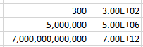
For the number 300 to be expressed in
exponential notation, Excel moves the decimal from after the whole number
300.00 to between the 3 and the 00. This is typed out as E+02 since the decimal
was moved two places to the left. The other examples are similar, where the
decimal was moved 6 and 12 places to the left.
Examples with small numbers, where the decimal is moved to the right:
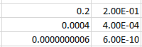
For the number 0.2 to be expressed in
exponential notation, Excel moves the decimal to create a whole number 2. This
is typed out as E-01 since the decimal was moved one place to the right. The
other examples are similar, where the decimal was moved 4 and 10 places to the
right.
Scientific formatting options are listed in the “Format Cells” dialog box, accessible by going to the “Home” tab of the ribbon, and clicking the “More Number Formats” option of the “Number Format” dropdown list.
The only option available is to alter the
number of decimal places shown in the number prior to the scientific notation.
For example, for the value 11.43 formatted with the scientific format, if we change the Decimal places from 2 to 1, the display will change as follows.
Two decimals: 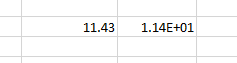
One decimal: 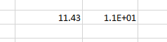
10- Text format
Cells can be formatted as Text through the
“Number Format” dropdown list, in the “Number” group of commands of the “Home”
tab.
Using the Text format in Excel allows values to be entered as they are, without Excel changing them per the above formatting rules.
In general, when entering a text in a cell, you won’t need to set its type to “Text”, as the default format type “General” is sufficient in most cases.
This may be useful when you want to display numbers with leading zeros, want to have spaces before or after numbers or letters, or when you want to display symbols that Excel normally uses for formulas.
Below are examples of some fields formatted as Text.
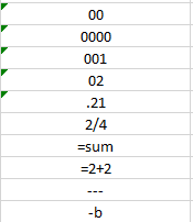
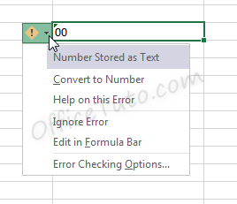
Note that when a number is formatted as Text, Excel will display a symbol showing that there could be a possible error ![]() .
.
Clicking the cell, then clicking the pop-up icon will show what the error may be and offer suggestions for resolution.
11- Special format
Special format offers four options in the “Format Cells” dialog box, accessible by going to the “Home” tab of the ribbon, and clicking the launcher arrow in the “Number” group of commands.
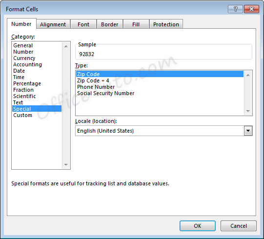
- Zip Code
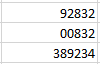
When less than five numbers are entered in Zip
Code format, leading zeros will be added to bring the total to five numbers.
When more than five numbers are entered in Zip Code format, all numbers will be displayed, even though this does not meet the format criteria.
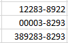
- Zip Code + 4
Zip Code + 4 format automatically creates a
dash symbol – before the last four numbers in the zip code.
When less than nine numbers are entered in Zip
Code + 4 format, leading zeros will be added to bring the total to nine
numbers.
When more than nine numbers are entered in Zip Code + 4 format, extra numbers are displayed prior to the dash symbol –.
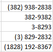
- Phone Number
Phone Number format automatically creates a
dash –
before the last four numbers in the phone number. This format also adds
parentheses ( ) around the area code when an area code is entered.
When less than the expected number of digits
are entered in Phone Number format, only the entered digits will be displayed,
starting from the end of the phone number, as shown on the third and fourth
lines, below.
When more than the expected number of digits
are entered in Phone Number format, extra numbers are displayed within the area
code parentheses.
Note that Phone Number format in Excel does not handle the number 1 before an area code. This entry would be treated like any other extra number.
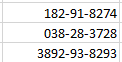
- Social Security Number
Social Security Number format automatically
creates a dash – before the last four numbers in the social security number
and a dash before the last six numbers in the social security number.
When less than nine numbers are entered in
Social Security Number format, leading zeros will be added to bring the total
to nine numbers.
When more than nine numbers are entered in Social Security Number format, extra numbers are displayed prior to the first dash –.
12- Custom format
Custom formats can be used or added through the
“Format Cells” dialog box, accessible from the “Number” group of commands in
the “Home” tab of the ribbon by clicking the “Number Format” launcher arrow.
This can be useful if the above formatting options do not work for your needs. Custom number formats can be created or updated by typing into the “Type” field of the “Format Cells” dialog box.
When creating a new custom format, be sure to use an existing custom format that you are okay with changing.
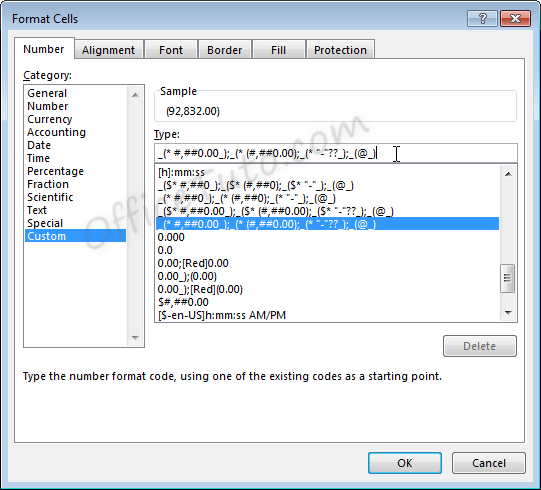
Custom number formats are separated, at
maximum, into four parts separated by semicolons ; .
- Part 1: How
to handle positive number values - Part 2: How
to handle negative number values - Part 3: How
to handle zero number values - Part 4: How
to handle text values
Note that if fewer parts are included in the custom format coding, Excel will determine how best to merge the above options: As an example, if two parts are listed, positive and zero values will be grouped.
Note that Excel may update the formatting of some fields to Custom automatically depending on what actions are taken on the field.
C- Common issues caused by wrong cell format types in Excel
1- Common issues due to wrong cell format types in Excel
The most common problems you may encounter with a wrong cell format type in Excel are of 3 types:
– Getting a wrong value.
– Getting an error.
– Formula displayed as-is and not calculated.
Let’s illustrate these 3 cases with some examples:
- Getting a wrong value
This may occur when you enter a value in an already formatted cell with an inappropriate format type, or when you apply a different format to a cell already containing a value.
The following table details some examples:
- Getting an error
This occurs when you enter a text preceded with a symbol of a dash, or plus, or equal, as an element of a list.
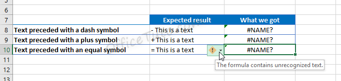
Excel wrongly interprets the text as a formula and show the error “The formula contains unrecognized text”.
- Formula displayed as-is and not calculated
In the following example, we tried to calculate the total of prices from cell B2 to B6 using the Excel SUM function, but Excel doesn’t calculate our formula and just displayed it as-is.
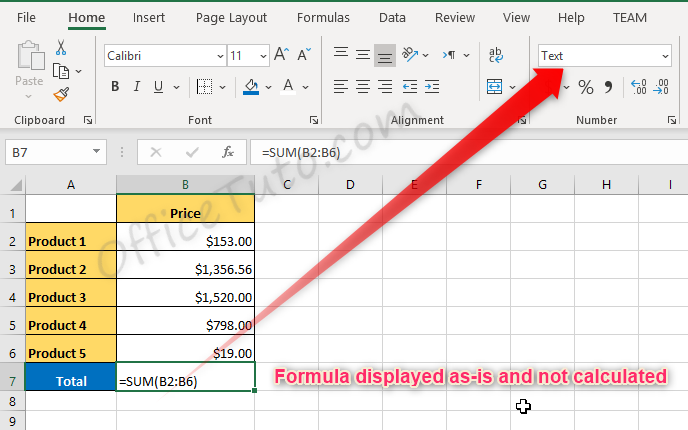
The source of the problem is that the result cell, B7, was previously formatted as text before entering the formula.
2- How to correct wrong cell format type issues in Excel
To correct cell format type issues in Excel, apply the right format in the “Number Format” drop-down list, and sometimes, you’ll also need to re-enter the content of the cell. For cells with formulas displayed as text, choose the “General” format, then double click in the cell and press Enter.

Jeff Golden is an experienced IT specialist and web publisher that has worked in the IT industry since 2010, with a focus on Office applications.
On this website, Jeff shares his insights and expertise on the different Office applications, especially Word and Excel.
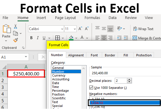
Definition of Format Cells
A format in excel can be defined as the change of appearance of the data in the cell the way it is, without changing the actual data or numbers in the cells. That means the data in the cell remains the same, but we will change the way it looks.
Different Formats in Excel
We have multiple formats in Excel to use. To see the available formats in excel, click on the “Home” menu on the top left corner.
General Format
In General format, there is no specific format; whatever you input, it will appear in the same way; it may be a number or text or symbol. After clicking on the HOME menu, go to the “NUMBER” segment, where you can find a drop of formats.
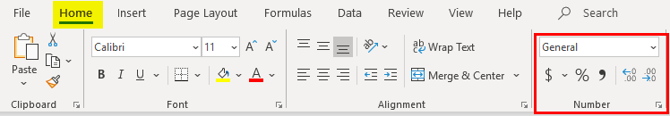
Click on the drop-down where you see the “General” option.
We will discuss each of these formats one by one with related examples.
1. Number Format
This format converts the data to a number format. When we input the data initially, it will be in General format; after converting to Number format only, it will appear as number format. Observe the below screenshot for the number in General format.
Now choose the format “Number” from the drop-down list and see how the appearance of cell A1 changes.
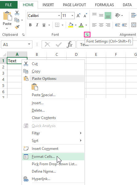
That is a difference between the General and Number format. If you want further customizations to your number format, select the cell that you want to do customization and right-click the below menu will come.
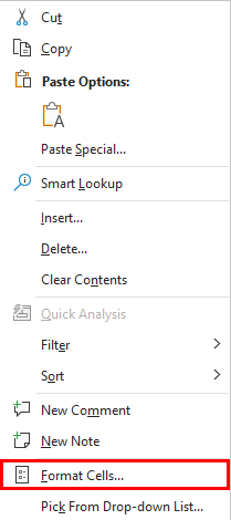
Choose the “Format Cells“ option then you will get the below window.
Choose “Number” under the “Category” option then you will get the customizations for the Number format. Choose the number of decimals you want to display. Tick the checkbox “Use 1000 separator” for separation of 1000’s with a comma (,).
Choose the negative number format whether you want to display with a negative symbol, brackets, red colour, nd red col, etc.
2. Currency Format
Currency format helps to convert the data to a currency format. We have an option to choose the type of currency as per our requirement. Select the cell which you want to convert to Currency format and choose the “Currency” option from the drop-down.
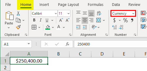
Currently, it is in Dollar currency. We can change by clicking on the drop-down of “$” and choose your required currency.
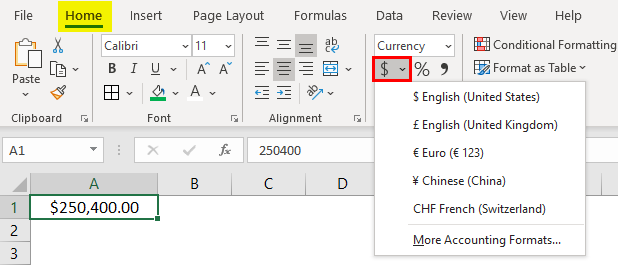
In the drop-down, we have few currencies; if you want the other currencies, click on the option “More Accounting formats”, which will display a pop-up menu as below.
Click on the drop-down “Symbol” and choose the required currency format.
3. Accounting Format
As you all know, accounting numbers are all related to money; hence whenever we convert any number to accounting format, it will add a currency symbol to that. The difference between currency and accounting is currency symbol alignment. Below are the screenshots for reference.
4. Accounting Alignment
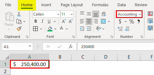
5. Currency Alignment
6. Short Date Format
A date can represent in a short format and long format. When you want to represent your date in a short format, use the short date format. E.g., 1/1/2019.
7. Long Date Format
The long date is used to represent our date in an expandable format like the below screenshot.
We see the short date format and long date format have multiple formats to represent our dates. Right-click and select “Format Cells” as to how we did before for “numbers”, then we will get the window to select the required formats.
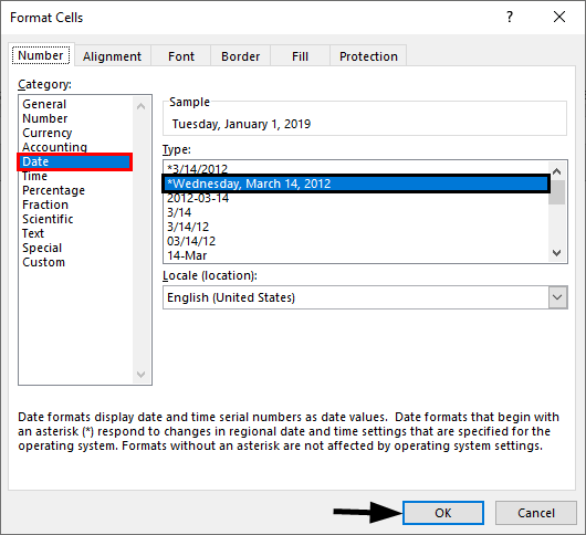
You can choose the location from the “Locale” drop-down menu.
Choose the date format under the “Type” menu.
We can represent our date in any of the formats from the available formats.
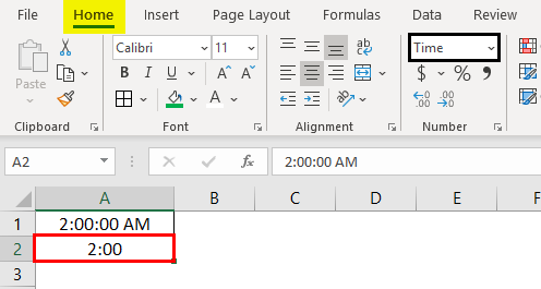
8. Time Format
This format is used to represent the time. If you input time without converting the cell into time format, it will show normally, but if you convert the cell into time format and input, it will clearly represent the time. Find the below screenshot for the differences.
If you still want to change the time format, then change in the format cells menu as shown below.
9. Percentage Format
Suppose you want to represent the number percentage use this format. Input any number in the cell and select that cell and choose the percentage format then the number will convert into a percentage.
10. Fraction Format
When we input the fraction numbers like 1/5, we should convert the cells into Fraction format. If we input the same 1/5 in a normal cell, it will show as a date.

This is how the fraction format works.
11. Text Format
When you input the number and convert it to text format, the number will align to the left side. It will consider as text as only, not the number.
12. Scientific Format
When you input a number 10000 (Ten thousand) and convert it into a scientific format, it will display as 1E+04, here E means exponent and 04 represents the number of zeros. If we input the number 0.0003, it will display as 3E-04. Try different numbers in excel format and check you will get a better idea to understand this better.
13. Other Formats
Apart from the explained formats, we have other formats like Alignment, Font, Border, Fill, and Protection.
Most of them are self-explanatory; hence I am leaving and explaining protection alone. When you want to lock any cells in the spreadsheet, use this option. But this lock will enable only when you protect the sheet.
You can hide and lock the cells on the same screen; Excel has provided instructions on when it will affect.
Things to Remember About Format Cells in Excel
- One can apply formats by right-clicking and selecting the format cells or from the drop-down as explained initially. The impact of them is the same; however, you will have multiple options when you right-click.
- When you want to apply a format to another cell, use format painter, select the cell, click on formatted painters, and choose the cell you want to apply.
- Use the option “Custom” when you want to create your own formats as per requirement.
Recommended Articles
This is a guide to Format Cells in Excel. Here we discuss how to format cells in excel along with practical examples and a downloadable excel template. You can also go through our other suggested articles to learn more–
- Excel Conditional Formatting for Dates
- Auto Format in Excel
- Formatting Text in Excel
- Excel Format Phone Numbers
When you fill out Excel worksheets with data, no one will succeed at once, everything is beautiful and correctly filled at the first attempt.
In the process of working with the program, you always need something: modify, edit, delete, copy or move. If the entered incorrect values in a cell, naturally, we want to correct or delete ones. But even such simple task can sometimes create difficulties.
How to set the cell format in Excel?
The contents of each Excel cell consist of three elements:
- The meaning: text, numbers, dates and times, logical content, functions and formulas.
- The formats: the type and color of the borders, the type and color of the fill, the way the values are displayed.
- Comments.
All these three elements are completely independent of each other. You can specify the format of the cell and do not write anything to it, or add a note in an empty and not formatted cell.
How to change the format of cells in Excel?
To change the format of the cells, you should call the corresponding dialog box with the CTRL + 1 (or CTRL + SHIFT + F) key or from the context menu after you right-click the «Cell Format» option.
There are 6 tabs in this dialog box:
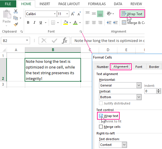
- A number. Here you specify the way the numeric values are displayed.
- The alignment. On this tab you can control the position of the text. And the text can be displayed vertically or diagonally from any angle. Also pay attention to the «Display» section. Very often, the function «Wrap Text» is used.
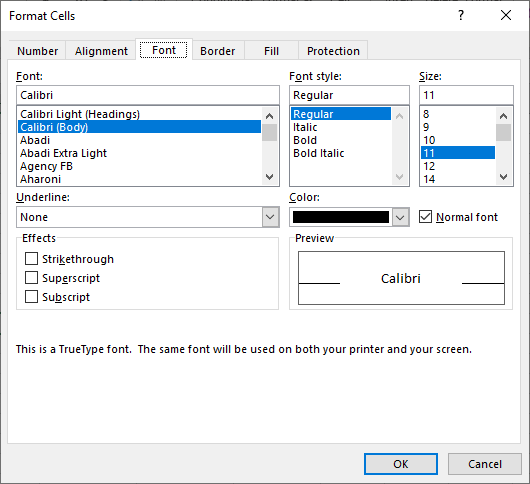
- Font. The specify the style design of fonts, the size and color of the text, plus the modes of modifications.
- The border. Here you define the styles and colors of the borders. The design of all tables is better done right here.
- The fill. The name of the bookmark speaks for itself. Available for formatting colors, patterns and methods of filling (for example, a gradient with a different direction of strokes).
- The protection. Here, the cell protection settings are set, that are activated only after the protection of the whole sheet.
If you did not get the desired result on the first attempt, call this dialog again to fix the cell format in Excel.
What formatting is applicable to cells in Excel?
Each cell always has some format. If there were no changes, then this is the «General» format. It is also a standard Excel format, in which:
- the numbers are aligned on the right side;
- the text is aligned on the left side;
- the font Calibri with the height of 11 points;
- the cell has no borders and background fill.
The Format Removal – is the changing to the standard «General» format (without borders and fills).
It is worth noting that the format of cells, unlike values, can not be deleted with the DELETE key.
To delete the format of cells, select ones and use the «Clear Formats» tool, which is located on the «HOME» tab in the «Editing» section.
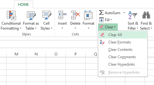
If you want to clear not only the format, but also the values, then select the «Clear All» option from the drop-down list of the tool (eraser).
As you can see, the eraser tool is functionally flexible and allows us to make a choice of what to delete in the cells:
- the content (same as the DELETE key);
- the formats;
- notes;
- the hyperlinks.
The option «Clear all» combines all these functions.
The deleting notes
Note, as well as formats, are not deleted from the cell by pressing the DELETE key. You can delete notes in two ways:
- The eraser tool: the option «Clear notes».
- Click on the cell with the note with the right mouse button, and from the appeared context menu select the option «Delete note».
The notation. The second way is more convenient. If you delete several notes at the same time, you must first select all of its cells.
Свойства ячейки, часто используемые в коде VBA Excel. Демонстрация свойств ячейки, как структурной единицы объекта Range, на простых примерах.
Объект Range в VBA Excel представляет диапазон ячеек. Он (объект Range) может описывать любой диапазон, начиная от одной ячейки и заканчивая сразу всеми ячейками рабочего листа.
Примеры диапазонов:
- Одна ячейка –
Range("A1"). - Девять ячеек –
Range("A1:С3"). - Весь рабочий лист в Excel 2016 –
Range("1:1048576").
Для справки: выражение Range("1:1048576") описывает диапазон с 1 по 1048576 строку, где число 1048576 – это номер последней строки на рабочем листе Excel 2016.
В VBA Excel есть свойство Cells объекта Range, которое позволяет обратиться к одной ячейке в указанном диапазоне (возвращает объект Range в виде одной ячейки). Если в коде используется свойство Cells без указания диапазона, значит оно относится ко всему диапазону активного рабочего листа.
Примеры обращения к одной ячейке:
Cells(1000), где 1000 – порядковый номер ячейки на рабочем листе, возвращает ячейку «ALL1».Cells(50, 20), где 50 – номер строки рабочего листа, а 20 – номер столбца, возвращает ячейку «T50».Range("A1:C3").Cells(6), где «A1:C3» – заданный диапазон, а 6 – порядковый номер ячейки в этом диапазоне, возвращает ячейку «C2».
Для справки: порядковый номер ячейки в диапазоне считается построчно слева направо с перемещением к следующей строке сверху вниз.
Подробнее о том, как обратиться к ячейке, смотрите в статье: Ячейки (обращение, запись, чтение, очистка).
В этой статье мы рассмотрим свойства объекта Range, применимые, в том числе, к диапазону, состоящему из одной ячейки.
Еще надо добавить, что свойства и методы объектов отделяются от объектов точкой, как в третьем примере обращения к одной ячейке: Range("A1:C3").Cells(6).
Свойства ячейки (объекта Range)
| Свойство | Описание |
|---|---|
| Address | Возвращает адрес ячейки (диапазона). |
| Borders | Возвращает коллекцию Borders, представляющую границы ячейки (диапазона). Подробнее… |
| Cells | Возвращает объект Range, представляющий коллекцию всех ячеек заданного диапазона. Указав номер строки и номер столбца или порядковый номер ячейки в диапазоне, мы получаем конкретную ячейку. Подробнее… |
| Characters | Возвращает подстроку в размере указанного количества символов из текста, содержащегося в ячейке. Подробнее… |
| Column | Возвращает номер столбца ячейки (первого столбца диапазона). Подробнее… |
| ColumnWidth | Возвращает или задает ширину ячейки в пунктах (ширину всех столбцов в указанном диапазоне). |
| Comment | Возвращает комментарий, связанный с ячейкой (с левой верхней ячейкой диапазона). |
| CurrentRegion | Возвращает прямоугольный диапазон, ограниченный пустыми строками и столбцами. Очень полезное свойство для возвращения рабочей таблицы, а также определения номера последней заполненной строки. |
| EntireColumn | Возвращает весь столбец (столбцы), в котором содержится ячейка (диапазон). Диапазон может содержаться и в одном столбце, например, Range("A1:A20"). |
| EntireRow | Возвращает всю строку (строки), в которой содержится ячейка (диапазон). Диапазон может содержаться и в одной строке, например, Range("A2:H2"). |
| Font | Возвращает объект Font, представляющий шрифт указанного объекта. Подробнее о цвете шрифта… |
| HorizontalAlignment | Возвращает или задает значение горизонтального выравнивания содержимого ячейки (диапазона). Подробнее… |
| Interior | Возвращает объект Interior, представляющий внутреннюю область ячейки (диапазона). Применяется, главным образом, для возвращения или назначения цвета заливки (фона) ячейки (диапазона). Подробнее… |
| Name | Возвращает или задает имя ячейки (диапазона). |
| NumberFormat | Возвращает или задает код числового формата для ячейки (диапазона). Примеры кодов числовых форматов можно посмотреть, открыв для любой ячейки на рабочем листе Excel диалоговое окно «Формат ячеек», на вкладке «(все форматы)». Свойство NumberFormat диапазона возвращает значение NULL, за исключением тех случаев, когда все ячейки в диапазоне имеют одинаковый числовой формат. Если нужно присвоить ячейке текстовый формат, записывается так: Range("A1").NumberFormat = "@". Общий формат: Range("A1").NumberFormat = "General". |
| Offset | Возвращает объект Range, смещенный относительно первоначального диапазона на указанное количество строк и столбцов. Подробнее… |
| Resize | Изменяет размер первоначального диапазона до указанного количества строк и столбцов. Строки добавляются или удаляются снизу, столбцы – справа. Подробнее… |
| Row | Возвращает номер строки ячейки (первой строки диапазона). Подробнее… |
| RowHeight | Возвращает или задает высоту ячейки в пунктах (высоту всех строк в указанном диапазоне). |
| Text | Возвращает форматированный текст, содержащийся в ячейке. Свойство Text диапазона возвращает значение NULL, за исключением тех случаев, когда все ячейки в диапазоне имеют одинаковое содержимое и один формат. Предназначено только для чтения. Подробнее… |
| Value | Возвращает или задает значение ячейки, в том числе с отображением значений в формате Currency и Date. Тип данных Variant. Value является свойством ячейки по умолчанию, поэтому в коде его можно не указывать. |
| Value2 | Возвращает или задает значение ячейки. Тип данных Variant. Значения в формате Currency и Date будут отображены в виде чисел с типом данных Double. |
| VerticalAlignment | Возвращает или задает значение вертикального выравнивания содержимого ячейки (диапазона). Подробнее… |
В таблице представлены не все свойства объекта Range. С полным списком вы можете ознакомиться не сайте разработчика.
Простые примеры для начинающих
Вы можете скопировать примеры кода VBA Excel в стандартный модуль и запустить их на выполнение. Как создать стандартный модуль и запустить процедуру на выполнение, смотрите в статье VBA Excel. Начинаем программировать с нуля.
Учтите, что в одном программном модуле у всех процедур должны быть разные имена. Если вы уже копировали в модуль подпрограммы с именами Primer1, Primer2 и т.д., удалите их или создайте еще один стандартный модуль.
Форматирование ячеек
Заливка ячейки фоном, изменение высоты строки, запись в ячейки текста, автоподбор ширины столбца, выравнивание текста в ячейке и выделение его цветом, добавление границ к ячейкам, очистка содержимого и форматирования ячеек.
Если вы запустите эту процедуру, информационное окно MsgBox будет прерывать выполнение программы и сообщать о том, что произойдет дальше, после его закрытия.
|
1 2 3 4 5 6 7 8 9 10 11 12 13 14 15 16 17 18 19 20 21 22 23 24 25 26 27 28 29 30 31 32 33 34 35 36 37 38 |
Sub Primer1() MsgBox «Зальем ячейку A1 зеленым цветом и запишем в ячейку B1 текст: «Ячейка A1 зеленая!»» Range(«A1»).Interior.Color = vbGreen Range(«B1»).Value = «Ячейка A1 зеленая!» MsgBox «Сделаем высоту строки, в которой находится ячейка A2, в 2 раза больше высоты ячейки A1, « _ & «а в ячейку B1 вставим текст: «Наша строка стала в 2 раза выше первой строки!»» Range(«A2»).RowHeight = Range(«A1»).RowHeight * 2 Range(«B2»).Value = «Наша строка стала в 2 раза выше первой строки!» MsgBox «Запишем в ячейку A3 высоту 2 строки, а в ячейку B3 вставим текст: «Такова высота второй строки!»» Range(«A3»).Value = Range(«A2»).RowHeight Range(«B3»).Value = «Такова высота второй строки!» MsgBox «Применим к столбцу, в котором содержится ячейка B1, метод AutoFit для автоподбора ширины» Range(«B1»).EntireColumn.AutoFit MsgBox «Выделим текст в ячейке B2 красным цветом и выровним его по центру (по вертикали)» Range(«B2»).Font.Color = vbRed Range(«B2»).VerticalAlignment = xlCenter MsgBox «Добавим к ячейкам диапазона A1:B3 границы» Range(«A1:B3»).Borders.LineStyle = True MsgBox «Сделаем границы ячеек в диапазоне A1:B3 двойными» Range(«A1:B3»).Borders.LineStyle = xlDouble MsgBox «Очистим ячейки диапазона A1:B3 от заливки, выравнивания, границ и содержимого» Range(«A1:B3»).Clear MsgBox «Присвоим высоте второй строки высоту первой, а ширине второго столбца — ширину первого» Range(«A2»).RowHeight = Range(«A1»).RowHeight Range(«B1»).ColumnWidth = Range(«A1»).ColumnWidth MsgBox «Демонстрация форматирования ячеек закончена!» End Sub |
Вычисления в ячейках (свойство Value)
Запись двух чисел в ячейки, вычисление их произведения, вставка в ячейку формулы, очистка ячеек.
Обратите внимание, что разделителем дробной части у чисел в VBA Excel является точка, а не запятая.
|
1 2 3 4 5 6 7 8 9 10 11 12 13 14 15 16 17 18 19 20 21 22 23 24 |
Sub Primer2() MsgBox «Запишем в ячейку A1 число 25.3, а в ячейку B1 — число 34.42» Range(«A1»).Value = 25.3 Range(«B1»).Value = 34.42 MsgBox «Запишем в ячейку C1 произведение чисел, содержащихся в ячейках A1 и B1» Range(«C1»).Value = Range(«A1»).Value * Range(«B1»).Value MsgBox «Запишем в ячейку D1 формулу, которая перемножает числа в ячейках A1 и B1» Range(«D1»).Value = «=A1*B1» MsgBox «Заменим содержимое ячеек A1 и B1 на числа 6.258 и 54.1, а также активируем ячейку D1» Range(«A1»).Value = 6.258 Range(«B1»).Value = 54.1 Range(«D1»).Activate MsgBox «Мы видим, что в ячейке D1 произведение изменилось, а в строке состояния отображается формула; « _ & «следующим шагом очищаем задействованные ячейки» Range(«A1:D1»).Clear MsgBox «Демонстрация вычислений в ячейках завершена!» End Sub |
Так как свойство Value является свойством ячейки по умолчанию, его можно было нигде не указывать. Попробуйте удалить .Value из всех строк, где оно встречается и запустить код заново.
Различие свойств Text, Value и Value2
Построение с помощью кода VBA Excel таблицы с результатами сравнения того, как свойства Text, Value и Value2 возвращают число, дату и текст.
|
1 2 3 4 5 6 7 8 9 10 11 12 13 14 15 16 17 18 19 20 21 22 23 24 25 26 27 28 29 30 31 32 33 34 35 36 37 38 39 40 41 42 43 44 45 46 47 48 49 50 51 52 53 54 55 56 |
Sub Primer3() ‘Присваиваем ячейкам всей таблицы общий формат на тот ‘случай, если формат отдельных ячеек ранее менялся Range(«A1:E4»).NumberFormat = «General» ‘добавляем сетку (границы ячеек) Range(«A1:E4»).Borders.LineStyle = True ‘Создаем строку заголовков Range(«A1») = «Значение» Range(«B1») = «Код формата» ‘формат соседней ячейки в столбце A Range(«C1») = «Свойство Text» Range(«D1») = «Свойство Value» Range(«E1») = «Свойство Value2» ‘Назначаем строке заголовков жирный шрифт Range(«A1:E1»).Font.Bold = True ‘Задаем форматы ячейкам A2, A3 и A4 ‘Ячейка A2 — числовой формат с разделителем триад и двумя знаками после запятой ‘Ячейка A3 — формат даты «ДД.ММ.ГГГГ» ‘Ячейка A4 — текстовый формат Range(«A2»).NumberFormat = «# ##0.00» Range(«A3»).NumberFormat = «dd.mm.yyyy» Range(«A4»).NumberFormat = «@» ‘Заполняем ячейки A2, A3 и A4 значениями Range(«A2») = 2362.4568 Range(«A3») = CDate(«01.01.2021») ‘Функция CDate преобразует текстовый аргумент в формат даты Range(«A4») = «Озеро Байкал» ‘Заполняем ячейки B2, B3 и B4 кодами форматов соседних ячеек в столбце A Range(«B2») = Range(«A2»).NumberFormat Range(«B3») = Range(«A3»).NumberFormat Range(«B4») = Range(«A4»).NumberFormat ‘Присваиваем ячейкам C2-C4 значения свойств Text ячеек A2-A4 Range(«C2») = Range(«A2»).Text Range(«C3») = Range(«A3»).Text Range(«C4») = Range(«A4»).Text ‘Присваиваем ячейкам D2-D4 значения свойств Value ячеек A2-A4 Range(«D2») = Range(«A2»).Value Range(«D3») = Range(«A3»).Value Range(«D4») = Range(«A4»).Value ‘Присваиваем ячейкам E2-E4 значения свойств Value2 ячеек A2-A4 Range(«E2») = Range(«A2»).Value2 Range(«E3») = Range(«A3»).Value2 Range(«E4») = Range(«A4»).Value2 ‘Применяем к таблице автоподбор ширины столбцов Range(«A1:E4»).EntireColumn.AutoFit End Sub |
Результат работы кода:

В таблице наглядно видна разница между свойствами Text, Value и Value2 при применении их к ячейкам с отформатированным числом и датой. Свойство Text еще отличается от Value и Value2 тем, что оно предназначено только для чтения.
What Is Excel Format Cells?
Formatting cells in Excel is one of the key options used to format the data. We can format data in different formats, such as time, date, currency, font, etc.,
For example, using format cells in excel, we can format time. If the value is 1800 hrs and we want to format it based on hh:mm AM/PM format, we can use the format cells option. As soon as we click format, the 1800 hrs will be formatted into 06:00 PM.
Table of contents
- What Is Excel Format Cells?
- How To Format Cells In Excel?
- Examples
- Important Things To Remember
- Frequently Asked Questions (FAQs)
- Recommended Articles
- Format cells in excel are used to format the data in the worksheet to present well and to save time.
- The tabs available in the Format cells option in excel are number, alignment, font, border, fill, and protection.
- Using the Number tab, we can format values such as date, currency, time, percentage, fraction, scientific notation, accounting number, etc., in excel.
- The shortcut keys to format date (in dd-mm-yy format) are Ctrl+Shift+#.
- Similarly, the shortcut keys to format time in hh:mm AM/PM format is [email protected]
How To Format Cells In Excel?
Formatting cells in excel is really simple. Let us have a look at the following examples to learn how to use format cells in excel.
You can download this Format Cell Excel Template here – Format Cell Excel Template
Examples
Example #1 – Format Date Cell
Excel stores date and time as serial numbers. We need to apply an appropriate format to the cell to see the date and time correctly.
For example, look at the below data.

It looks like a serial number to us, but we get date values when applying date format in excel to these serial numbers.
The date has a wide variety of formats. Below is a list of formats we can apply to dates.

We can apply any formatting codes to see the date, as shown above in the respective format.
- To apply the date format, we must first select the range of cells and press Ctrl + 1 to open the format window. Then, under Custom, we must apply the code as we want to see the date.
Format Cells Shortcut Key
![]()

We get the following result.

Example #2 – Format Time Cell
As we said, the date and time are stored as serial numbers in Excel. Now, it is time to see the TIME formatting in excel. For example, look at the numbers below.

The TIME values are varied from 0 to less than 0.99999, so let us apply the time format to see the time. Below are the time format codes we can generally use:
“h:mm:ss”
To apply the time format, we must follow the same steps:

So, we get the following result.

So, the number “0.70192” equals the time of 16:50:46.
If we do not want to see the time in the 24-hour format, we need to apply the time formatting code like the one below.

Now, we will get the result as shown in the below image.

Now, our time is shown as 04:50:46 PM instead of 16:50:46.
Example #3 – Format Date And Time Together
The date and time are together in Excel. We can format both the date and time together in Excel. For example, look at the below data.

Let us apply the date and time format to these cells to see the results. The formatting code is dd-mmm-yyyy hh:mm:ss AM/PM.

We get the following result.

Let us analyze this briefly now.
The first value we had was 43689.6675 for this, we have applied the date and time format as dd-mm-yyyy hh:mm:ss AM/PM, so the result is 12-Aug-2019 04:01:12 PM.
43689 represents data in this number, and the decimal value 0.6675021991 represents time.
Example #4 – Positive And Negative Values
When dealing with numbers, positive and negative values are part of it. To differentiate between these two values by showing them with different colors is the general rule everybody follows. For example, look at the below data.

To apply a number format to these numbers and show negative red values, below is the code.

“#,###;[Red]-#,###”
If we apply this formatting code, we can see the above numbers.

Similarly, showing negative numbers in brackets is also in practice. For example, to show the negative numbers in the bracket and red color, below is the code.
“#,###;[Red](-#,###)”

We get the following result.

Example #5 – Add Suffix Words To Numbers
If we want to add suffix words along with numbers and still be able to do calculations, it is great.
If we show a person’s weight, adding the suffix word KG will add more value to the numbers. Below is the person’s weight in KG.

To show this data with the suffix word KG, apply the below formatting code.
### ” KG”

After applying the code, the weight column looks like as shown below.

Example #6 – Using Format Painter
Format Painter Excel, we can apply one cell format to another. For example, look at the below image.

The date format is DD-MM-YYYY, and the remaining cells are not formatted for the first cell. But, we can apply the format of the first cell to the remaining cells by using a format painter.
We must select the first cell, then go to the Home tab and click on Format Painter.

Now, we must click on the next cell to apply the formatting.

Now again, select the cell and apply the formatting, but this is not the smart way of using a format painter. Instead, double-click on Format Painter by selecting the cell. Once we double-click, we can apply the format to any number of cells, applying all at once.

Important Things To Remember
- The format option is used to format the data in different formats.
- We can format the date and time together.
- The Excel Format Painter is the tool used to copy one cell format to another.
Frequently Asked Questions (FAQs)
1. What are format cells in excel?
Format cells is an option used to format the values used in excel.
We can use the format cells option by clicking on
Home → Cells group → Format drop-down option → Format Cells
2. How to format data in excel?
We can format the date with simple steps;
Consider the following example. The date of birth of 3 people is in 3 different formats. Now, let us learn how to format the date such that cell range B2:B4 are in the same format.

The steps used to format date are:
• Step 1: Select cell B2.
• Step 2: Select Home → Cells group → Format drop-down option → Format Cells
• Step 3: The Format Cells tab pops up.

• Step 4: Click Date from the Category under Number tab.

• Step 5: We can select the desired option. In our example, let us select the 4th option.
As we click OK¸ we can see that the value in cell B2 is formatted.

Similarly, we can format cells in excel.
3. What are the shortcut keys to format cells in excel?
The following are some useful shortcut keys to format cells in excel:
• Ctrl+Shift+~ – General Format
• Ctrl+Shift+# – Format Date
• [email protected] – Format Time
Recommended Articles
This article is a guide to Format cells in Excel. Here, we discuss the top 6 tips to format cells, including date, time, date and time together, format painter, etc., examples, and a downloadable Excel template. You may also look at these useful functions in Excel: –
- Shortcut Key to Start New Line in Excel Cell
- Export Excel into PDF File
- How to Format Phone Numbers in Excel?
- Accounting Number Excel Format