
Change the format of a cell
You can apply formatting to an entire cell and to the data inside a cell—or a group of cells. One way to think of this is the cells are the frame of a picture and the picture inside the frame is the data.

Formal Cells
-
Select the cells.
-
Go to the ribbon to select changes as Bold, Font Color, or Font Size.
Apply Excel Styles
-
Select the cells.
-
Select Home > Cell Style and select a style.
Modify an Excel Style
-
Select the cells with the Excel Style.
-
Right-click the applied style in Home > Cell Styles.
-
Select Modify > Format to change what you want.
Need more help?
You can always ask an expert in the Excel Tech Community or get support in the Answers community.
See Also
Format text in cells
Format numbers
Format a date the way you want
Need more help?
Want more options?
Explore subscription benefits, browse training courses, learn how to secure your device, and more.
Communities help you ask and answer questions, give feedback, and hear from experts with rich knowledge.
![]()
Download Article
![]()
Download Article
Knowing how to format your spreadsheet in Excel, the cells in particular, can really help you improve not just the aesthetic perspective of your document, but also its effectiveness in providing relevant information to the viewers of the files. Each cell in Microsoft Excel can be modified and formatted to follow your specific preferences.
-

1
Open your Microsoft Excel. Click the “Start” button on the lower-left corner of your screen and select “All Programs” from the menu. Inside, you’ll find the “Microsoft Office” folder where Excel is listed. Click on Excel.
-
2
Select the specific cell or group of cells that you want to format. Highlight it using your mouse cursor.
Advertisement
-
3
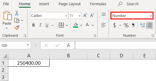
Open the Format Cells window. Right-click on the cells you’ve selected and select “Format Cells” from the pop up menu to access the “Format Cells” window.
-
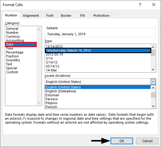
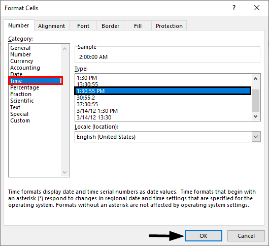
4
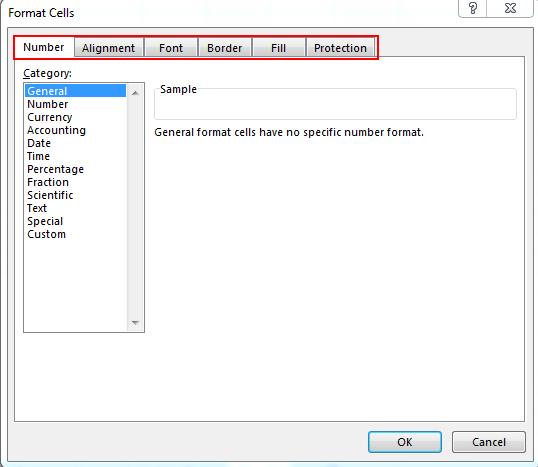
Set the desired formatting options you want for the cell. There are six formatting options that you can use to customize a cell or group of cells:
- Number – Defines the format of numerical data entered on the cells such as dates, currency, time, percentage, fraction and more.
- Alignment – Sets how the data will be visually aligned inside each cells (left, right or centered).
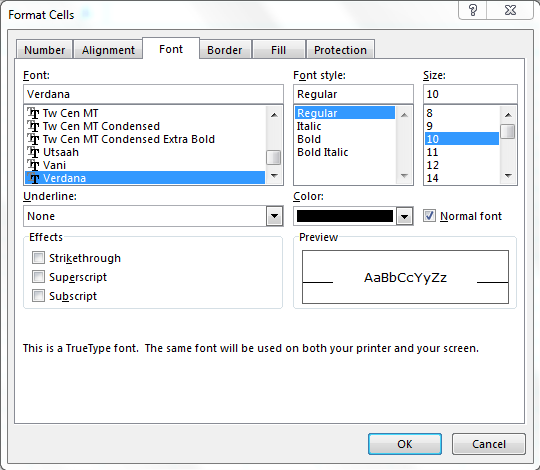
- Font – Sets all the options related to text fonts such as styles, sizes and colors.
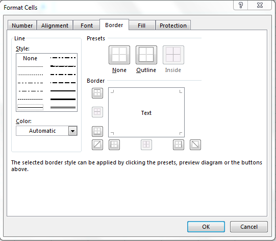
- Border – Improves the visual appearance of each cell by adding definite lines (borders) around a cell or group of cells.
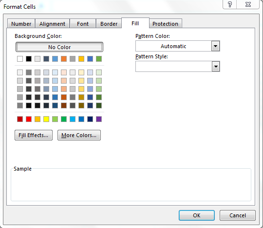
- Fill – Sets the background color and pattern formats of each cell on the spreadsheet.
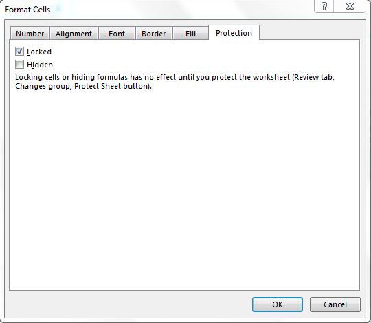
- Protection – Adds security to cells and data contained inside it by hiding or locking the selected cells or group of cells.
-
5
Save. Click on the “OK” button at the lower right corner of the “Format Cells” window to save any changes you’ve made and apply the formats you’ve set to the selected cells.


Advertisement
Ask a Question
200 characters left
Include your email address to get a message when this question is answered.
Submit
Advertisement
-
Avoid using formats that are visually irritating such as fill colors that don’t compliment the colors of the fonts, or artistic font styles that are not appropriate for formal documents like the spreadsheet.
-
You can use this method to format cells of new files or existing spreadsheet documents you currently have.
-
When formatting cells in Excel, do it in groups (either by rows or columns) so that your spreadsheet will have a clean and uniform appearance.
Thanks for submitting a tip for review!
Advertisement
About This Article
Article SummaryX
To format a cell in Microsoft Excel, start by highlighting the specific cell you want to format. Then, right-click on the cell and click on «Format Cells.» Choose whatever formatting you want for the cell from the different options, then click «Okay.» That’s all there is to it! For a step-by-step walkthrough with pictures, check out the full article below!
Did this summary help you?
Thanks to all authors for creating a page that has been read 72,532 times.
Is this article up to date?
What Is Excel Format Cells?
Formatting cells in Excel is one of the key options used to format the data. We can format data in different formats, such as time, date, currency, font, etc.,
For example, using format cells in excel, we can format time. If the value is 1800 hrs and we want to format it based on hh:mm AM/PM format, we can use the format cells option. As soon as we click format, the 1800 hrs will be formatted into 06:00 PM.
Table of contents
- What Is Excel Format Cells?
- How To Format Cells In Excel?
- Examples
- Important Things To Remember
- Frequently Asked Questions (FAQs)
- Recommended Articles
- Format cells in excel are used to format the data in the worksheet to present well and to save time.
- The tabs available in the Format cells option in excel are number, alignment, font, border, fill, and protection.
- Using the Number tab, we can format values such as date, currency, time, percentage, fraction, scientific notation, accounting number, etc., in excel.
- The shortcut keys to format date (in dd-mm-yy format) are Ctrl+Shift+#.
- Similarly, the shortcut keys to format time in hh:mm AM/PM format is [email protected]
How To Format Cells In Excel?
Formatting cells in excel is really simple. Let us have a look at the following examples to learn how to use format cells in excel.
You can download this Format Cell Excel Template here – Format Cell Excel Template
Examples
Example #1 – Format Date Cell
Excel stores date and time as serial numbers. We need to apply an appropriate format to the cell to see the date and time correctly.
For example, look at the below data.

It looks like a serial number to us, but we get date values when applying date format in excel to these serial numbers.
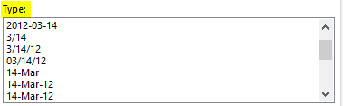
The date has a wide variety of formats. Below is a list of formats we can apply to dates.

We can apply any formatting codes to see the date, as shown above in the respective format.
- To apply the date format, we must first select the range of cells and press Ctrl + 1 to open the format window. Then, under Custom, we must apply the code as we want to see the date.
Format Cells Shortcut Key
![]()

We get the following result.

Example #2 – Format Time Cell
As we said, the date and time are stored as serial numbers in Excel. Now, it is time to see the TIME formatting in excel. For example, look at the numbers below.

The TIME values are varied from 0 to less than 0.99999, so let us apply the time format to see the time. Below are the time format codes we can generally use:
“h:mm:ss”
To apply the time format, we must follow the same steps:

So, we get the following result.

So, the number “0.70192” equals the time of 16:50:46.
If we do not want to see the time in the 24-hour format, we need to apply the time formatting code like the one below.

Now, we will get the result as shown in the below image.

Now, our time is shown as 04:50:46 PM instead of 16:50:46.
Example #3 – Format Date And Time Together
The date and time are together in Excel. We can format both the date and time together in Excel. For example, look at the below data.

Let us apply the date and time format to these cells to see the results. The formatting code is dd-mmm-yyyy hh:mm:ss AM/PM.

We get the following result.

Let us analyze this briefly now.
The first value we had was 43689.6675 for this, we have applied the date and time format as dd-mm-yyyy hh:mm:ss AM/PM, so the result is 12-Aug-2019 04:01:12 PM.
43689 represents data in this number, and the decimal value 0.6675021991 represents time.
Example #4 – Positive And Negative Values
When dealing with numbers, positive and negative values are part of it. To differentiate between these two values by showing them with different colors is the general rule everybody follows. For example, look at the below data.

To apply a number format to these numbers and show negative red values, below is the code.

“#,###;[Red]-#,###”
If we apply this formatting code, we can see the above numbers.

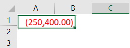
Similarly, showing negative numbers in brackets is also in practice. For example, to show the negative numbers in the bracket and red color, below is the code.
“#,###;[Red](-#,###)”

We get the following result.

Example #5 – Add Suffix Words To Numbers
If we want to add suffix words along with numbers and still be able to do calculations, it is great.
If we show a person’s weight, adding the suffix word KG will add more value to the numbers. Below is the person’s weight in KG.

To show this data with the suffix word KG, apply the below formatting code.
### ” KG”

After applying the code, the weight column looks like as shown below.

Example #6 – Using Format Painter
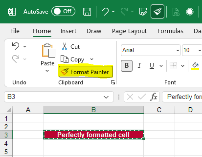
Format Painter Excel, we can apply one cell format to another. For example, look at the below image.

The date format is DD-MM-YYYY, and the remaining cells are not formatted for the first cell. But, we can apply the format of the first cell to the remaining cells by using a format painter.
We must select the first cell, then go to the Home tab and click on Format Painter.

Now, we must click on the next cell to apply the formatting.

Now again, select the cell and apply the formatting, but this is not the smart way of using a format painter. Instead, double-click on Format Painter by selecting the cell. Once we double-click, we can apply the format to any number of cells, applying all at once.

Important Things To Remember
- The format option is used to format the data in different formats.
- We can format the date and time together.
- The Excel Format Painter is the tool used to copy one cell format to another.
Frequently Asked Questions (FAQs)
1. What are format cells in excel?
Format cells is an option used to format the values used in excel.
We can use the format cells option by clicking on
Home → Cells group → Format drop-down option → Format Cells
2. How to format data in excel?
We can format the date with simple steps;
Consider the following example. The date of birth of 3 people is in 3 different formats. Now, let us learn how to format the date such that cell range B2:B4 are in the same format.

The steps used to format date are:
• Step 1: Select cell B2.
• Step 2: Select Home → Cells group → Format drop-down option → Format Cells
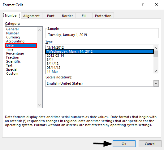
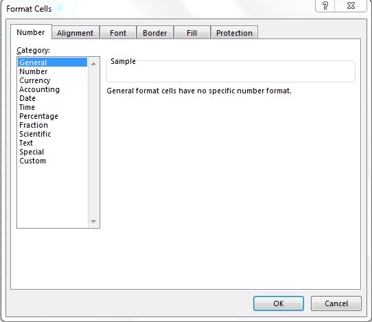
• Step 3: The Format Cells tab pops up.

• Step 4: Click Date from the Category under Number tab.

• Step 5: We can select the desired option. In our example, let us select the 4th option.
As we click OK¸ we can see that the value in cell B2 is formatted.

Similarly, we can format cells in excel.
3. What are the shortcut keys to format cells in excel?
The following are some useful shortcut keys to format cells in excel:
• Ctrl+Shift+~ – General Format
• Ctrl+Shift+# – Format Date
• [email protected] – Format Time
Recommended Articles
This article is a guide to Format cells in Excel. Here, we discuss the top 6 tips to format cells, including date, time, date and time together, format painter, etc., examples, and a downloadable Excel template. You may also look at these useful functions in Excel: –
- Shortcut Key to Start New Line in Excel Cell
- Export Excel into PDF File
- How to Format Phone Numbers in Excel?
- Accounting Number Excel Format
This tutorial about cell format types in Excel is an essential part of your learning of Excel and will definitely do a lot of good to you in your future use of this software, as a lot of tasks in Excel sheets are based on cells format, as well as several errors are due to a bad implementation of it.
A good comprehension of the cell format types will build your knowledge on a solid basis to master Excel basics and will considerably save you time and effort when any related issue occurs.
A- Introduction
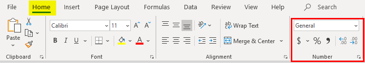
Excel software formats the cells depending on what type of information they contain.
To update the format of the highlighted cell, go to the “Home” tab of the ribbon and click, in the “Number” group of commands on the “Number Format” drop-down list.
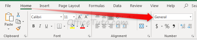
The drop-down list allows the selection to be changed.
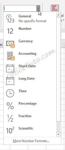
Cell formatting options in the “Number Format” drop-down list are:
- General
- Number
- Currency
- Accounting
- Short Date
- Long Date
- Time
- Percentage
- Fraction
- Scientific
- Text
- And the “More Number Formats” option.
Clicking the “More Number Formats” option brings up additional options for formatting cells, including the ability to do special and custom formatting options.
These options are discussed in detail in the below sections.
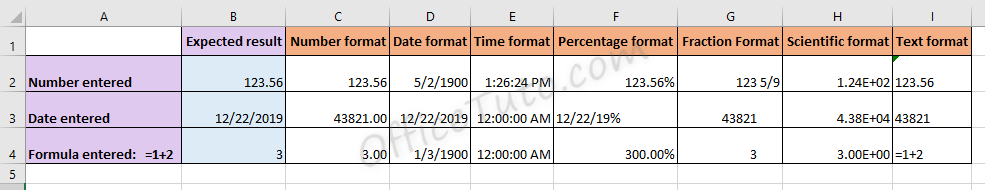
Cell format types in Excel are: General, Number, Currency, Accounting, Date, Time, Percentage, Fraction, Scientific, Text, Special (Zip Code, Zip Code + 4, Phone Number, Social Security Number), and Custom. You can get them from the “Number Format” drop-down list in the “Home” tab, or from the launcher arrow below it.
I will detail each one of them in the following sections:
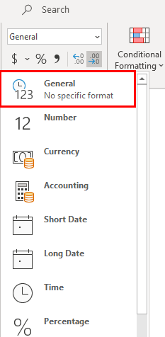
1- General format
By default, cells are formatted as “General”, which could store any type of information. The General format means that no specific format is applied to the selected cell.
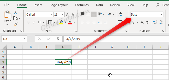
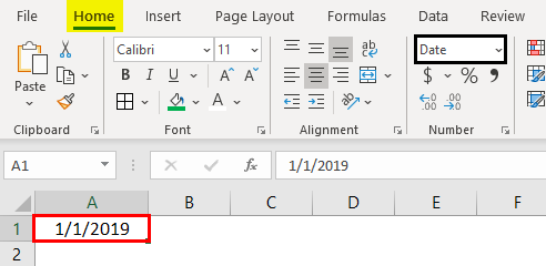
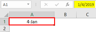
When information is typed into a cell, the cell format may change automatically. For example, if I enter “4/4/19” into a cell and press enter, then highlight the cell to view details about it, the cell format will be listed as “Date” instead of “General”.
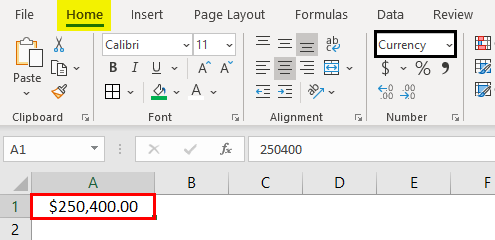
Similarly, we can update a cell’s format before or after entering data to adjust the way the data appears. Changing the format of a cell to “Currency” will make it so information entered is displayed as a dollar amount.
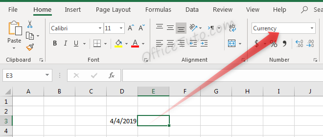
Typing a number into this cell and pressing enter will not just show that number, but will instead format it accordingly.
Before pressing enter, Excel shows the value which was typed: “4”.
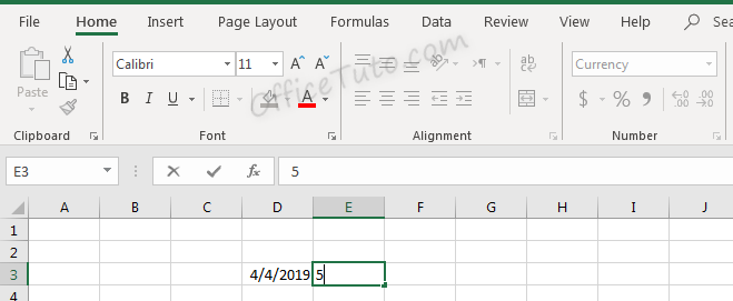
After pressing enter, the value is updated based on the formatting type selected.
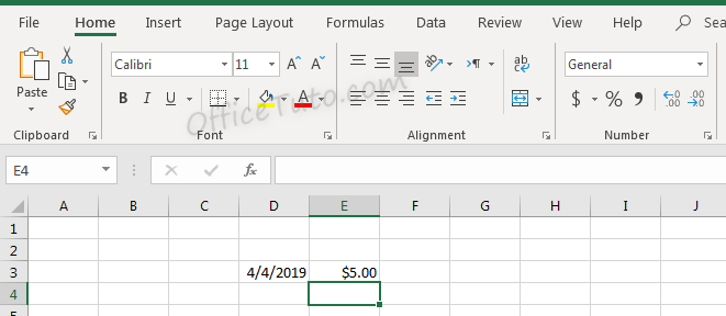
Don’t let the format type showed in the illustration at the drop-down list confusing you; it is reflecting the cell below (i.e. E4), since we validated by an Enter.
2- Number format
Cells formatted as numbers behave differently than general formatted cells. By default, when a number is entered, or when a cell is formatted as a number already, the alignment of the information within the cell will be on the right instead of on the left. This makes it easier to read a list of numbers such as the below.
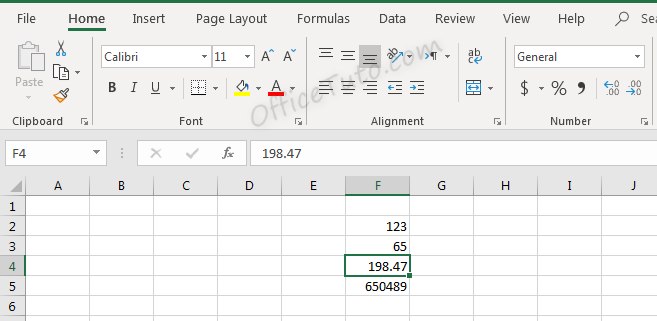
Note in the above screenshot that since we didn’t choose the “Number” format for our cells, they still have a “General” one. They are numbers for Excel (meaning, we can do calculations on them), but they didn’t have yet the number format and its formatting aspects:
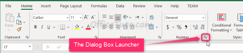
You can set the formatting options for Excel numbers in the “Format Cells” dialog box.
To do that, select the cell or the range of cells you want to set the formatting options for their numbers, and go to the “Home” tab of the ribbon, then in the “Number” group of commands, click on the launcher of the dialog box (the arrow on the right-down side of the group).
Excel opens the “Format Cells” dialog box in its “Number” tab. Click in the “Category” pane on “Number”.
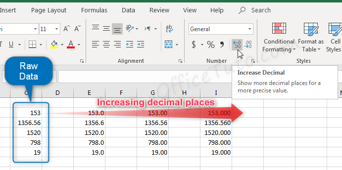
- In this dialog box, you can decide how many decimal places to display by updating options in the “Decimal places” field.
Note that this feature is also available in the “Home” tab of the ribbon where you can go to the “Number” group of commands and click the Increase Decimal ![]() or Decrease Decimal
or Decrease Decimal ![]() buttons.
buttons.
Here is the result of consecutive increasing of decimal places on our example of data (1 decimal; 2 decimals; and 3 decimals):
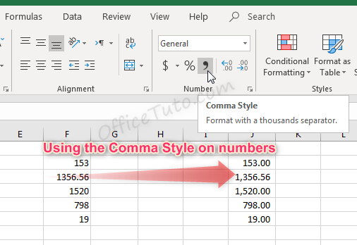
- You can also decide if commas should be shown in the display as a thousand separator, by updating the “Use 1000 Separator (,)” option in the “Format Cells” dialog box.
This feature is also available in the “Home” tab of the ribbon by clicking the “Comma Style” button ![]() in the “Number” group of commands.
in the “Number” group of commands.
Note that using the Comma Style button will automatically set the format to Accounting.
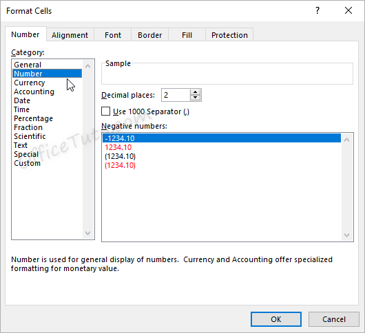
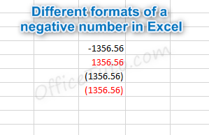
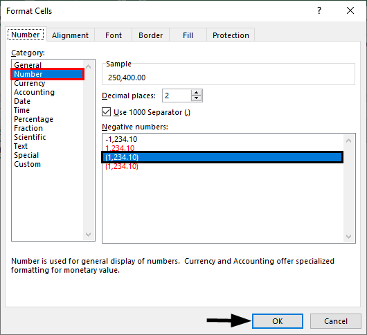
- Another option from the Format Cells dialog box is to decide how negative numbers should display by using the “Negative numbers” field.
There are four options for displaying negative
numbers.
- Display
negative numbers with a negative sign before the number. - Display
negative numbers in red. - Display
negative numbers in parentheses. - Display
negative numbers in red and in parentheses.
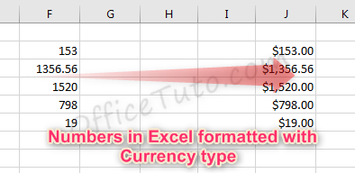
3- Currency format
Cells formatted as currency have a currency symbol such as a dollar sign $ immediately to the left of the number in the cell, and contain two numbers after the decimal by default.
The alignment of numbers in currency formatted cells will be on the right for readability.
Currency formatting options are similar to
number formatting options, apart from the currency symbol display.
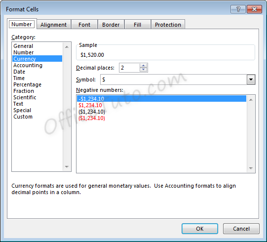
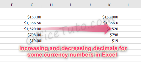
- As with regular number formatting, you can decide, in the “Format Cells” dialog box, how many decimal places to display by updating the field “Decimal places”.
You can also find this feature in the “Home” tab of the ribbon, by going to the “Number” group of commands and clicking the Increase Decimal ![]() or Decrease Decimal
or Decrease Decimal ![]() .
.
- You can also decide what currency symbol should be shown in the display by updating the “Symbol” field in the “Format Cells” dialog box.
- As with regular number formatting, you can also decide how negative numbers should display by updating the “Negative numbers” field in the “Format Cells” dialog box.
There are four
options for displaying negative numbers.
- Display
negative numbers with a negative sign before the number. - Display
negative numbers in red. - Display
negative numbers in parentheses. - Display
negative numbers in red and in parentheses.
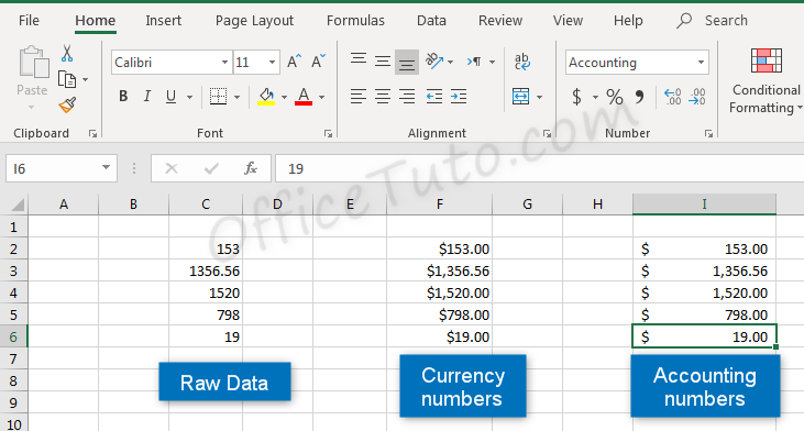
4- Accounting format
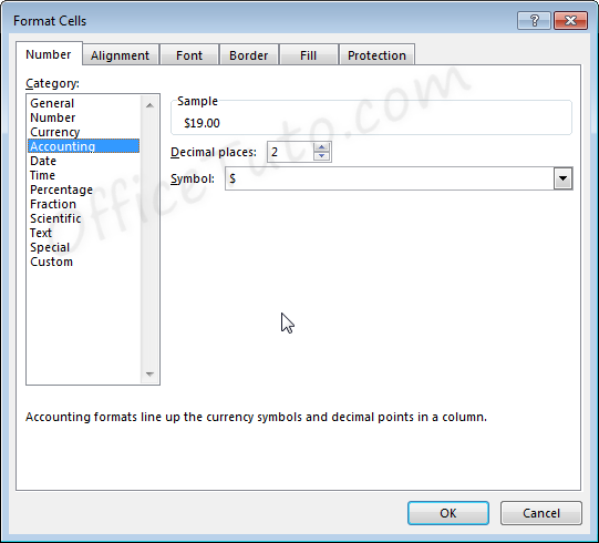
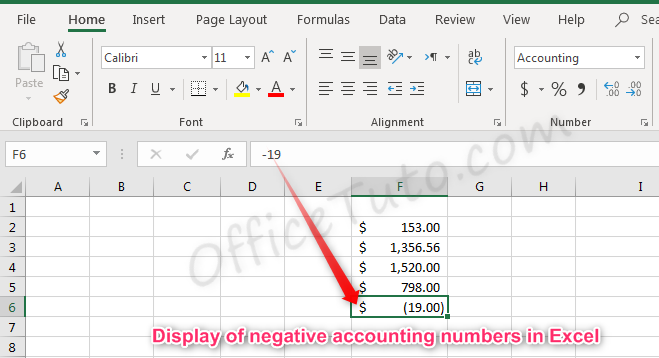
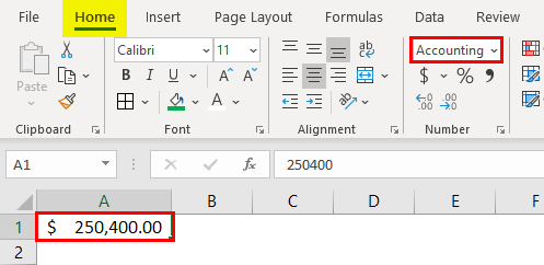
Like with the currency format, cells formatted as accounting have a currency symbol such as a dollar sign $; however, this symbol is to the far left of the cell, while the alignment of numbers in the cell is on the right. Accounting numbers contain two numbers after the decimal by default.
Clicking the “Accounting Number Format” button ![]() in the “Number” group of commands of the “Home” tab, will quickly format a cell or cells as Accounting.
in the “Number” group of commands of the “Home” tab, will quickly format a cell or cells as Accounting.
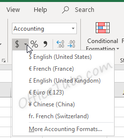
The down arrow to the right of the Accounting Number Format button allows selection between common symbols used for accounting, including English (dollar sign), English (pound), Euro, Chinese, and French symbols.
Accounting formatting options in the “Format Cells” dialog box (“Home” tab of the ribbon, in the “Number” group of commands, click on the launcher of the “Number Format” dialog box), are similar to number and currency formatting options.
- You can decide how many decimal places to display by updating its option in the “Format Cells” dialog box.
As mentioned before in this tutorial, this feature is also available directly in the “Home” tab of the ribbon by clicking the Increase Decimal ![]() or Decrease Decimal
or Decrease Decimal ![]() buttons in the “Number” group of commands.
buttons in the “Number” group of commands.
- You can also decide in the “Format Cells” dialog box, what currency symbol should be shown in the display by using the “Symbol” drop-down list.
This dropdown gives a much broader list of options than the “Accounting Number Format” option in the “Home” tab of the ribbon.
Note that with the Accounting formatting option, negative numbers display in parentheses by default. There are not options to change this.
5- Date format
There are options for “Short Date” and “Long Date” in the “Number Format” dropdown list of the “Home” tab.
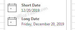
Short date shows the date with slashes separating month, day, and year. The order of the month and day may vary depending on your computer’s location settings.
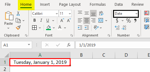
Long date shows the date with the day of the week, month, day, and year separated by commas.
More options for formatting dates are available in the “Format Cells” dialog box (accessible by clicking in the “Number Format” dropdown list of the “Home” tab and choosing the “More Number Formats” option at the bottom).
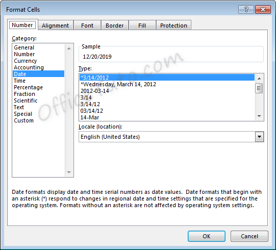
- You can choose from a long list of available date formats.
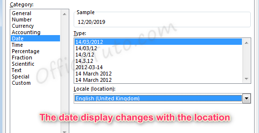
- You can update the location settings used for formatting the date. This will alter the list of format options in the above list and will adjust the display and potentially the order of the elements (day, month, year) within the date.
Note the below example when we switch from English (United States) format to English (United Kingdom) format.
6- Time format
Cells formatted as time display the time of
day. The default time display is based on your computer’s location settings.
Time formatting options are available in the “Format Cells” dialog box (accessible by choosing the “More Number Formats” option at the bottom of the “Number Format” dropdown list in the “Home” tab of the ribbon).
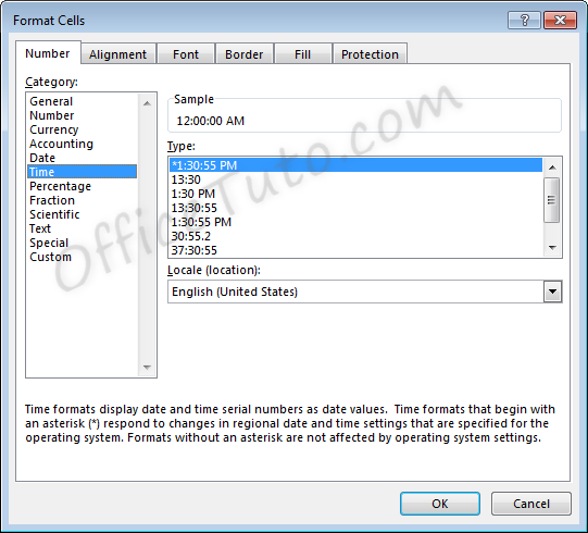
- You can choose from a long list of available time formats.
- You can update the location settings used for formatting the time. This will alter the list of format options in the above list and will adjust the display.
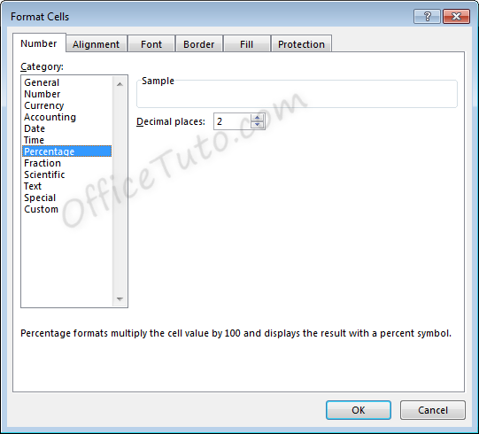
7- Percentage format
Cells formatted as percentage display a percent sign to the right of the number. You can change the format of a cell to a percentage using the “Number Format” dropdown list, or by clicking the “Percent Style” button ![]() . Both options are accessible from the “Home” tab of the ribbon, in the “Number” group of commands.
. Both options are accessible from the “Home” tab of the ribbon, in the “Number” group of commands.
Note that updating a number to a percentage
will expect that the number already contains the decimal. For example:
A cell containing the value 0.08, as a percentage, will show 8%.
A cell containing the value 8, as a percentage, will show 800%.
Percentage formatting options are available in the “Format Cells” dialog box, accessible by clicking on “More Number Formats” of the “Number Format” dropdown list in the “Home” tab of the ribbon.
8- Fraction format
Cells formatted as a fraction display with a slash
symbol separating the numerator and denominator.
Fraction formatting options are available in the “Format Cells” dialog box, accessible by clicking in the “Home” tab of the ribbon, on “More Number Formats” of the “Number Format” dropdown list.
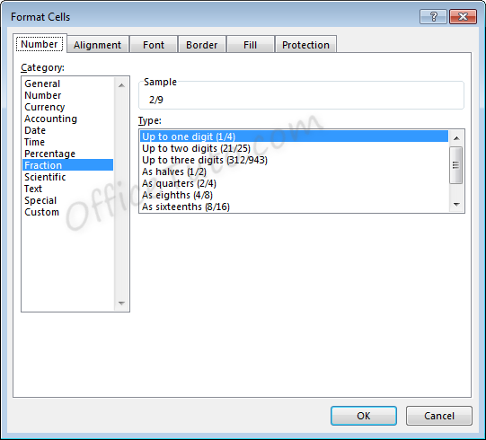
- Note that
when selecting the format to use for a fraction, Excel will round to the
nearest fraction where the formatting criteria can be met.
As an example, if the
formatting option selected is “Up to one digit”, entering a fraction with two
digits will cause rounding to occur. For example, with the setting of “Up to
one digit”,
If we enter a value of 7/16, the value displayed will be 4/9, as converting to 9ths was the option with only one digit which required the least amount of rounding.
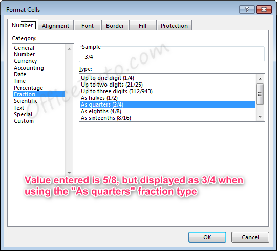
For another example, if the formatting option selected is “As quarters”, entering a fraction that cannot be expressed in quarters (divisible by four) will also cause rounding to occur.
If we enter a value of 5/8, the value displayed will be 3/4. Excel rounded up to 6/8, or 3/4, which was the closest option divisible by four.
- Also note
that for the formatting options with “Up to x digits”, Excel will always round
down to the lowest exact equivalent fraction when possible.
For example, if we enter a value of 2/4 with one of these formatting options active, the value displayed will be 1/2, as this is the mathematical equivalent. This behavior will not take place for formatting options “As…”, since these specifically determine what the denominator should be.
- Fractions listed as more than a whole (meaning the numerator is a higher number than the denominator), such as 7/4 will automatically be adjusted into a whole number and a fraction 13/4, where the fraction follows the formatting rules selected.
9- Scientific format
Scientific format, otherwise known as
Exponential Notation, allows very large and small numbers to be accurately
represented within a cell, even when the size of the cell cannot accommodate
the size of the numbers.
The way exponential notation works is to theoretically place a decimal in a spot that would make the number shorter, then describe where to move that decimal to return to the original number.
Examples with large numbers, where the decimal is moved to the left:
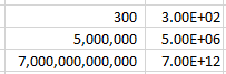
For the number 300 to be expressed in
exponential notation, Excel moves the decimal from after the whole number
300.00 to between the 3 and the 00. This is typed out as E+02 since the decimal
was moved two places to the left. The other examples are similar, where the
decimal was moved 6 and 12 places to the left.
Examples with small numbers, where the decimal is moved to the right:
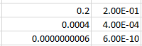
For the number 0.2 to be expressed in
exponential notation, Excel moves the decimal to create a whole number 2. This
is typed out as E-01 since the decimal was moved one place to the right. The
other examples are similar, where the decimal was moved 4 and 10 places to the
right.
Scientific formatting options are listed in the “Format Cells” dialog box, accessible by going to the “Home” tab of the ribbon, and clicking the “More Number Formats” option of the “Number Format” dropdown list.
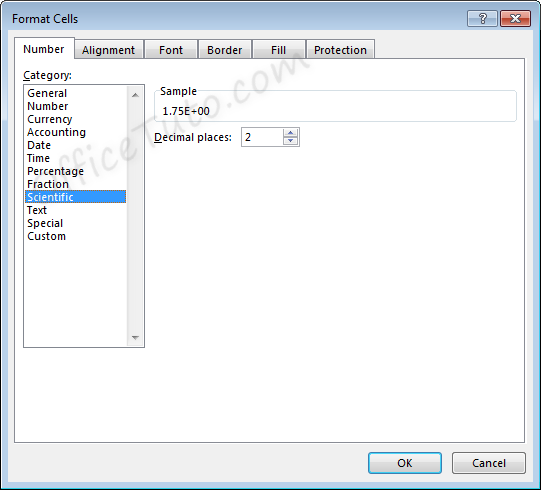
The only option available is to alter the
number of decimal places shown in the number prior to the scientific notation.
For example, for the value 11.43 formatted with the scientific format, if we change the Decimal places from 2 to 1, the display will change as follows.
Two decimals: 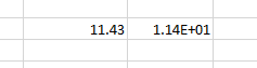
One decimal: 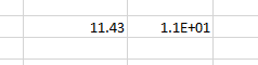
10- Text format
Cells can be formatted as Text through the
“Number Format” dropdown list, in the “Number” group of commands of the “Home”
tab.
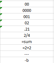
Using the Text format in Excel allows values to be entered as they are, without Excel changing them per the above formatting rules.
In general, when entering a text in a cell, you won’t need to set its type to “Text”, as the default format type “General” is sufficient in most cases.
This may be useful when you want to display numbers with leading zeros, want to have spaces before or after numbers or letters, or when you want to display symbols that Excel normally uses for formulas.
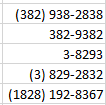
Below are examples of some fields formatted as Text.
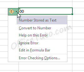
Note that when a number is formatted as Text, Excel will display a symbol showing that there could be a possible error ![]() .
.
Clicking the cell, then clicking the pop-up icon will show what the error may be and offer suggestions for resolution.
11- Special format
Special format offers four options in the “Format Cells” dialog box, accessible by going to the “Home” tab of the ribbon, and clicking the launcher arrow in the “Number” group of commands.
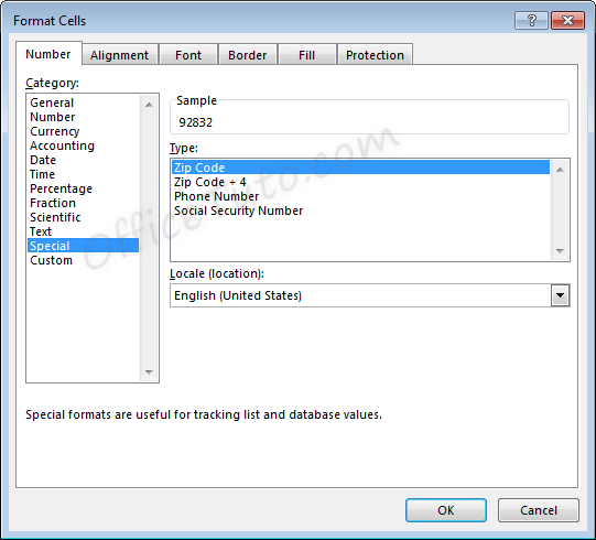
- Zip Code
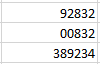
When less than five numbers are entered in Zip
Code format, leading zeros will be added to bring the total to five numbers.
When more than five numbers are entered in Zip Code format, all numbers will be displayed, even though this does not meet the format criteria.
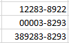
- Zip Code + 4
Zip Code + 4 format automatically creates a
dash symbol – before the last four numbers in the zip code.
When less than nine numbers are entered in Zip
Code + 4 format, leading zeros will be added to bring the total to nine
numbers.
When more than nine numbers are entered in Zip Code + 4 format, extra numbers are displayed prior to the dash symbol –.
- Phone Number
Phone Number format automatically creates a
dash –
before the last four numbers in the phone number. This format also adds
parentheses ( ) around the area code when an area code is entered.
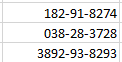
When less than the expected number of digits
are entered in Phone Number format, only the entered digits will be displayed,
starting from the end of the phone number, as shown on the third and fourth
lines, below.
When more than the expected number of digits
are entered in Phone Number format, extra numbers are displayed within the area
code parentheses.
Note that Phone Number format in Excel does not handle the number 1 before an area code. This entry would be treated like any other extra number.
- Social Security Number
Social Security Number format automatically
creates a dash – before the last four numbers in the social security number
and a dash before the last six numbers in the social security number.
When less than nine numbers are entered in
Social Security Number format, leading zeros will be added to bring the total
to nine numbers.
When more than nine numbers are entered in Social Security Number format, extra numbers are displayed prior to the first dash –.
12- Custom format
Custom formats can be used or added through the
“Format Cells” dialog box, accessible from the “Number” group of commands in
the “Home” tab of the ribbon by clicking the “Number Format” launcher arrow.
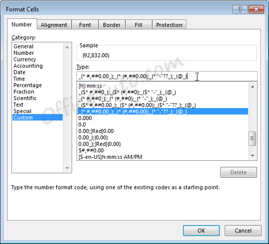
This can be useful if the above formatting options do not work for your needs. Custom number formats can be created or updated by typing into the “Type” field of the “Format Cells” dialog box.
When creating a new custom format, be sure to use an existing custom format that you are okay with changing.
Custom number formats are separated, at
maximum, into four parts separated by semicolons ; .
- Part 1: How
to handle positive number values - Part 2: How
to handle negative number values - Part 3: How
to handle zero number values - Part 4: How
to handle text values
Note that if fewer parts are included in the custom format coding, Excel will determine how best to merge the above options: As an example, if two parts are listed, positive and zero values will be grouped.
Note that Excel may update the formatting of some fields to Custom automatically depending on what actions are taken on the field.
C- Common issues caused by wrong cell format types in Excel
1- Common issues due to wrong cell format types in Excel
The most common problems you may encounter with a wrong cell format type in Excel are of 3 types:
– Getting a wrong value.
– Getting an error.
– Formula displayed as-is and not calculated.
Let’s illustrate these 3 cases with some examples:
- Getting a wrong value
This may occur when you enter a value in an already formatted cell with an inappropriate format type, or when you apply a different format to a cell already containing a value.
The following table details some examples:
- Getting an error
This occurs when you enter a text preceded with a symbol of a dash, or plus, or equal, as an element of a list.
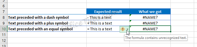
Excel wrongly interprets the text as a formula and show the error “The formula contains unrecognized text”.
- Formula displayed as-is and not calculated
In the following example, we tried to calculate the total of prices from cell B2 to B6 using the Excel SUM function, but Excel doesn’t calculate our formula and just displayed it as-is.
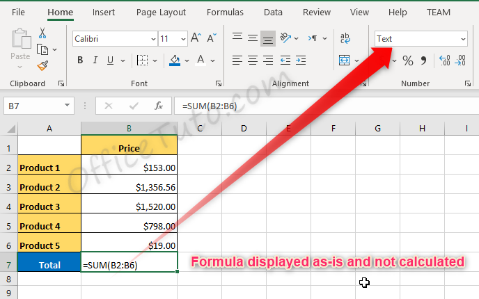
The source of the problem is that the result cell, B7, was previously formatted as text before entering the formula.
2- How to correct wrong cell format type issues in Excel
To correct cell format type issues in Excel, apply the right format in the “Number Format” drop-down list, and sometimes, you’ll also need to re-enter the content of the cell. For cells with formulas displayed as text, choose the “General” format, then double click in the cell and press Enter.

Jeff Golden is an experienced IT specialist and web publisher that has worked in the IT industry since 2010, with a focus on Office applications.
On this website, Jeff shares his insights and expertise on the different Office applications, especially Word and Excel.
Definition of Format Cells
A format in excel can be defined as the change of appearance of the data in the cell the way it is, without changing the actual data or numbers in the cells. That means the data in the cell remains the same, but we will change the way it looks.
Different Formats in Excel
We have multiple formats in Excel to use. To see the available formats in excel, click on the “Home” menu on the top left corner.
General Format
In General format, there is no specific format; whatever you input, it will appear in the same way; it may be a number or text or symbol. After clicking on the HOME menu, go to the “NUMBER” segment, where you can find a drop of formats.
Click on the drop-down where you see the “General” option.
We will discuss each of these formats one by one with related examples.
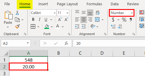
1. Number Format
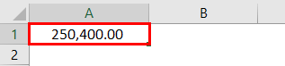
This format converts the data to a number format. When we input the data initially, it will be in General format; after converting to Number format only, it will appear as number format. Observe the below screenshot for the number in General format.
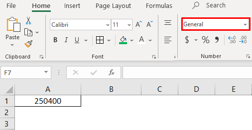
Now choose the format “Number” from the drop-down list and see how the appearance of cell A1 changes.
That is a difference between the General and Number format. If you want further customizations to your number format, select the cell that you want to do customization and right-click the below menu will come.
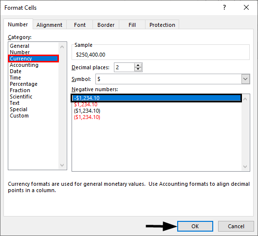
Choose the “Format Cells“ option then you will get the below window.
Choose “Number” under the “Category” option then you will get the customizations for the Number format. Choose the number of decimals you want to display. Tick the checkbox “Use 1000 separator” for separation of 1000’s with a comma (,).
Choose the negative number format whether you want to display with a negative symbol, brackets, red colour, nd red col, etc.
2. Currency Format
Currency format helps to convert the data to a currency format. We have an option to choose the type of currency as per our requirement. Select the cell which you want to convert to Currency format and choose the “Currency” option from the drop-down.
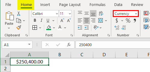
Currently, it is in Dollar currency. We can change by clicking on the drop-down of “$” and choose your required currency.
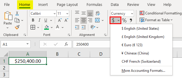
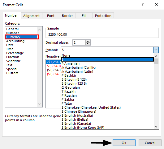
In the drop-down, we have few currencies; if you want the other currencies, click on the option “More Accounting formats”, which will display a pop-up menu as below.
Click on the drop-down “Symbol” and choose the required currency format.
3. Accounting Format
As you all know, accounting numbers are all related to money; hence whenever we convert any number to accounting format, it will add a currency symbol to that. The difference between currency and accounting is currency symbol alignment. Below are the screenshots for reference.
4. Accounting Alignment
5. Currency Alignment
6. Short Date Format
A date can represent in a short format and long format. When you want to represent your date in a short format, use the short date format. E.g., 1/1/2019.
7. Long Date Format
The long date is used to represent our date in an expandable format like the below screenshot.
We see the short date format and long date format have multiple formats to represent our dates. Right-click and select “Format Cells” as to how we did before for “numbers”, then we will get the window to select the required formats.
You can choose the location from the “Locale” drop-down menu.
Choose the date format under the “Type” menu.
We can represent our date in any of the formats from the available formats.
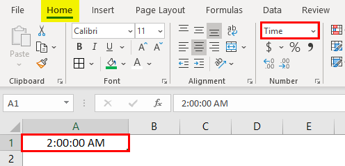
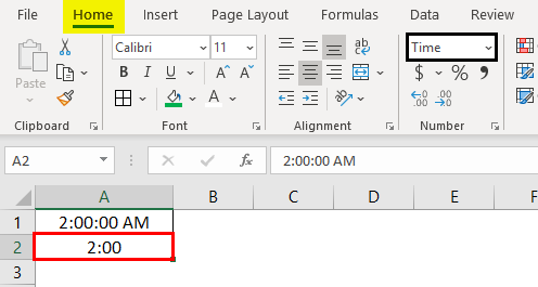
8. Time Format
This format is used to represent the time. If you input time without converting the cell into time format, it will show normally, but if you convert the cell into time format and input, it will clearly represent the time. Find the below screenshot for the differences.
If you still want to change the time format, then change in the format cells menu as shown below.
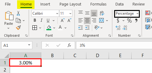
9. Percentage Format
Suppose you want to represent the number percentage use this format. Input any number in the cell and select that cell and choose the percentage format then the number will convert into a percentage.
10. Fraction Format
When we input the fraction numbers like 1/5, we should convert the cells into Fraction format. If we input the same 1/5 in a normal cell, it will show as a date.
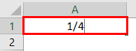

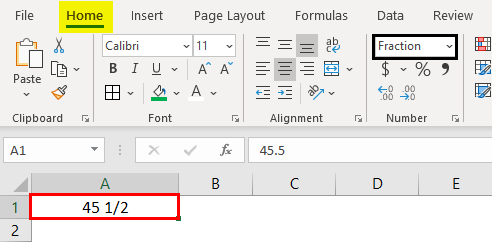
This is how the fraction format works.
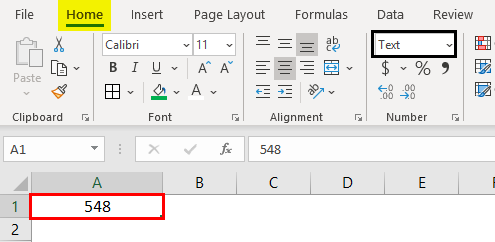
11. Text Format
When you input the number and convert it to text format, the number will align to the left side. It will consider as text as only, not the number.
12. Scientific Format
When you input a number 10000 (Ten thousand) and convert it into a scientific format, it will display as 1E+04, here E means exponent and 04 represents the number of zeros. If we input the number 0.0003, it will display as 3E-04. Try different numbers in excel format and check you will get a better idea to understand this better.
13. Other Formats
Apart from the explained formats, we have other formats like Alignment, Font, Border, Fill, and Protection.
Most of them are self-explanatory; hence I am leaving and explaining protection alone. When you want to lock any cells in the spreadsheet, use this option. But this lock will enable only when you protect the sheet.
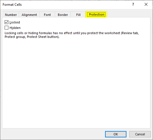
You can hide and lock the cells on the same screen; Excel has provided instructions on when it will affect.
Things to Remember About Format Cells in Excel
- One can apply formats by right-clicking and selecting the format cells or from the drop-down as explained initially. The impact of them is the same; however, you will have multiple options when you right-click.
- When you want to apply a format to another cell, use format painter, select the cell, click on formatted painters, and choose the cell you want to apply.
- Use the option “Custom” when you want to create your own formats as per requirement.
Recommended Articles
This is a guide to Format Cells in Excel. Here we discuss how to format cells in excel along with practical examples and a downloadable excel template. You can also go through our other suggested articles to learn more–
- Excel Conditional Formatting for Dates
- Auto Format in Excel
- Formatting Text in Excel
- Excel Format Phone Numbers
We use Format Cells to change the formatting of cell number without changing the number itself. We can use Format cells to change the number, alignment, font style, Border style, Fill options and Protection.
We can find this option with right click of the mouse. After right-clicking, pop-up will appear, and then we need to click on Format Cells or we can use shortcut key Ctrl+1 on our keyboard.
Format Cells: — Excel cell format option is used for changing the appearance of number without any changes in number. We can change font, protect the file, etc.
To formatting the cells there are five tabs in Format Cells. By using this, we can change the date style, time style, Alignments, insert the border with different style, protect the cells, etc.
Number Tab:-Excel number format used for changing the formatting of number cells in decimals, providing the desired format, in terms of number, dates, converting into percentage, fractions, etc.
Alignment Tab:-By using this tab, we can align the cell’s text, merge the two cell’s text with each other. If the text is hidden, then by using the wrap text, we can show it properly, and also we can align the text as per the desired direction.
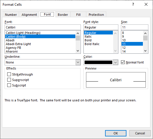
Font Tab: —By using this tab, we can change the font, font color, font style, font size, etc. We can underline the text, can change the font effects, and we can preview also how it would look like.
Border Tab: —By using this tab, we can create colorful border line to different type of styles; if we don’t want to provide the border outline, we can leave it blank.
Fill Tab: —By using this tab, we can fill the cell or range with colors in different types of styles, we can combine two colors, and also we can insert picture in a cell by using Fill option.
Protection Tab: —By using this tab, we can protect cell, range, formula containing cells, sheet, etc.
Let’s take a brief example to understand how we can use Format Cells:-
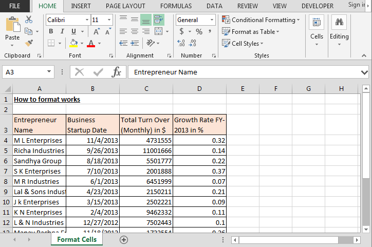
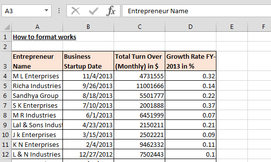
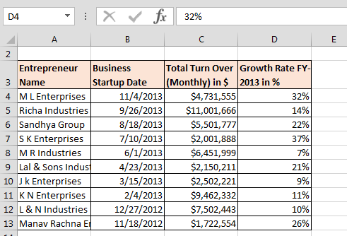
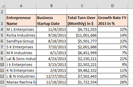
We have growth rate data with the turnover of various companies. In this data, we can see that headers are not visible properly, dates are not in proper format, turn over amount is in dollar but it’s not showing. Also, growth rate is not showing in %age format.
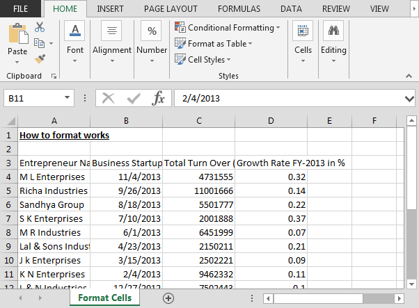
By using the format cell option, we will format the data in presentable manner.
How to make the viewable header of the report?
- Select the range A3:D3.
- Press the key Ctrl+1.
- Format cell dialog box will open.
- Go to Alignment tab.
- Select the Wrap text option (this option is used to adjust the text within a cell).
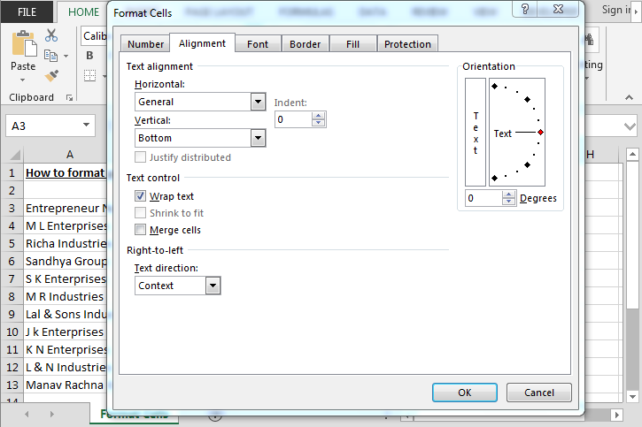
- Click on OK.

How to make the border?
- Select the data.
- Press the key Ctrl+1.
- Format cell dialog box will open.
- Go to border option.
- Click on the border line.
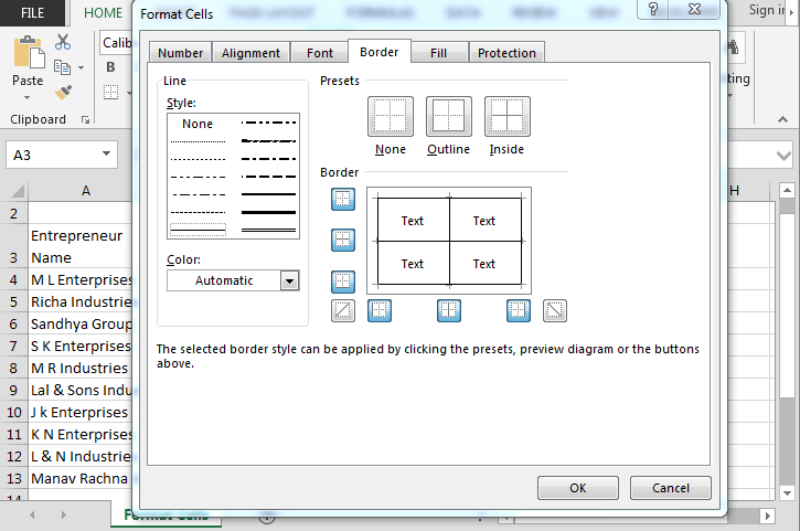
- Click on OK.

How to fill the color in header?
- Select the header.
- Press the key Ctrl+1.
- Format cell dialog box will open.
- Go to fill tab and select the color accordingly.
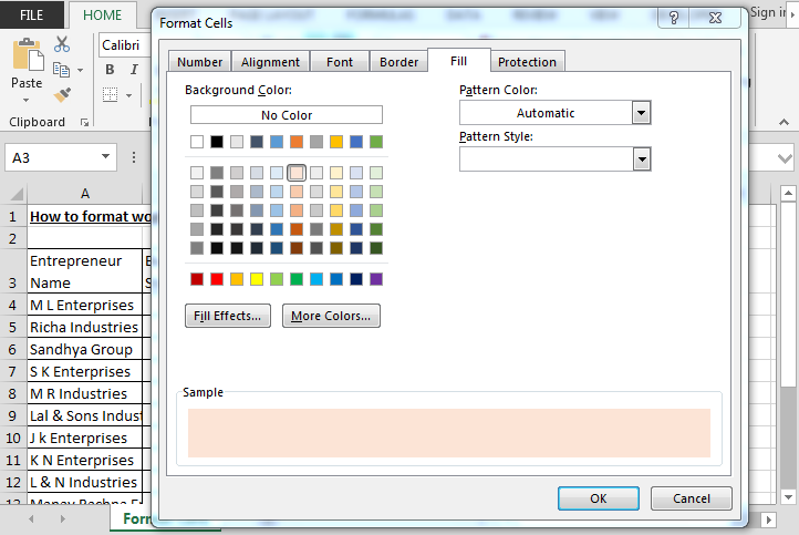
- Click on OK.
- Press the key Ctrl+B to make the header bold.
How to change numbers into currency format?
- Select the turnover column.
- Press the key Ctrl+1.
- Format cell dialog box will open.
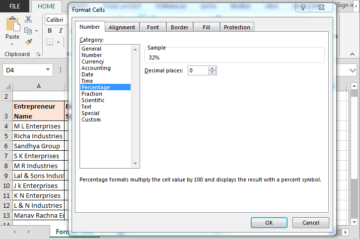
- Go to Number tab > Currency > Decimal places 0 and select the $ symbol.
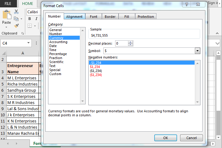
- Click on OK.
How to change numbers formatting into %age format?
- Select the Growth rate column.
- Press the key Ctrl+1.
- Format cell dialog box will open.
- Go to Number tab > Percentage > Decimal places 0.
- Click on OK.
Data before formatting:-

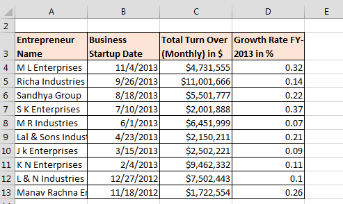
Data after formatting:-
This is the way to use of Format cells in Microsoft Excel.

Skip to content
Мы рассмотрим, какие форматы данных используются в Excel. Кроме того, расскажем, как можно быстро изменять внешний вид ячеек самыми различными способами.
Когда дело доходит до форматирования ячеек в Excel, большинство пользователей знают, как применять основные текстовые и числовые форматы. Но знаете ли вы, как отобразить необходимое количество десятичных знаков или определенный символ валюты, и как применить экспоненциальный или финансовый формат? А знаете ли вы, какие комбинации клавиш в Excel позволяют одним щелчком применить желаемое оформление? Почему Excel сам изменяет формат ячеек и как с этим бороться?
Итак, вот о чём мы сегодня поговорим:
- Что такое формат ячейки
- Способы настройки формата ячеек
- Как настроить параметры текста
- Комбинации клавиш для быстрого изменения формата
- Почему Excel не меняет формат ячейки?
- Как бороться с автоматическим форматированием?
- 4 способа копирования форматов
- Как создать и работать со стилями форматирования
Что такое формат данных в Excel?
По умолчанию все ячейки на листах Microsoft Excel имеют формат «Общий». При этом все, что вы вводите в них, обычно остается как есть (но не всегда).
В некоторых случаях Excel может отображать значение не именно так, как вы его ввели, хотя формат установлен как Общий. Например, если вы вводите большое число в узком столбце, Excel может отобразить его в научном формате, например, 4.7E + 08. Но если вы посмотрите в строке формул, вы увидите исходное число, которое вы ввели (470000000).
Бывают ситуации, когда Excel может автоматически изменить вид ваших данных в зависимости от значения, которое вы записали. Например, если вы введете 4/1/2021 или 1/4, Excel будет рассматривать это как дату и соответствующим образом изменит формат записи.
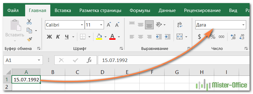
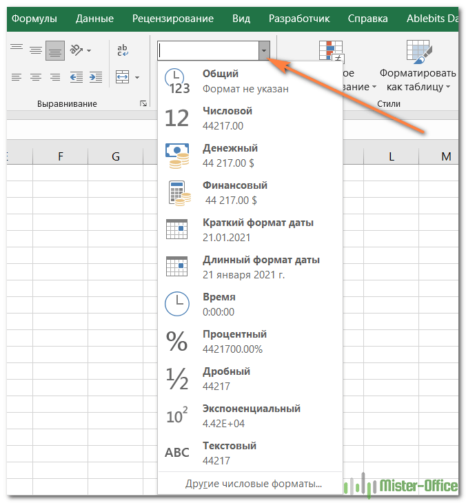
Самый простой способ проверить формат, примененный к определенной ячейке, – выбрать ее и посмотреть на поле Числовой формат на вкладке Главная:
Важно помнить, что форматирование в Excel изменяет только внешний вид или визуальное представление содержимого, но не само значение.
Например, если у вас есть число 0,6691, и вы настроите так, чтобы отображалось только 2 десятичных знака, то оно будет отображаться как 0,67. Но реальное значение не изменится, и Excel будет использовать 0,6691 во всех расчетах.
Точно так же вы можете изменить отображение значений даты и времени так, как вам нужно. Но Excel сохранит исходное значение (целое число для даты и десятичный остаток для времени) и будет использовать их во всех функциях даты и времени и других формулах.
Чтобы увидеть настоящее значение, скрытое за числовым форматом, выберите ячейку и посмотрите на строку формул:

Как настроить формат ячейки в Excel
Когда вы хотите изменить внешний вид числа или даты, отобразить границы ячеек, изменить выравнивание и направление текста или внести какие-либо другие изменения, диалоговое окно «Формат ячеек» является основной функцией, которую следует использовать. И поскольку это наиболее часто используемый инструмент для изменения представления данных в Excel, Microsoft сделала ее доступной множеством способов.
4 способа открыть диалоговое окно «Формат ячеек».
Чтобы изменить оформление данных в определенной позиции или диапазоне в Excel, прежде всего выберите то, вид чего вы хотите изменить. А затем выполните одно из следующих четырёх действий:
- Нажмите комбинацию
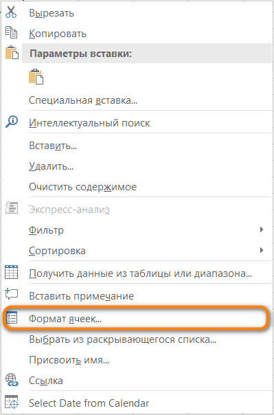
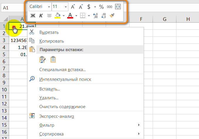
Ctrl + 1. - Щелкните правой кнопкой мыши (или нажмите
Shift + F10) и выберите нужный пункт во всплывающем меню.
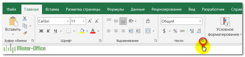
3. Щелкните стрелку запуска диалогового окна в правом нижнем углу группы Число.
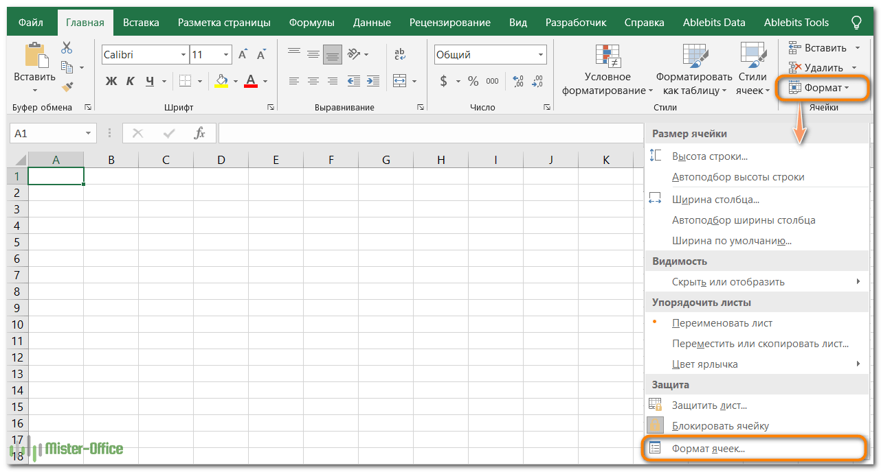
4. На вкладке «Главная» в группе «Ячейки» нажмите кнопку «Формат», а затем выберите «Формат ячеек».
Появится диалоговое окно, и вы сможете поменять отображение выбранных ячеек, используя различные параметры на любой из шести вкладок.
6 вкладок диалогового окна «Формат ячеек».
Эти вкладки содержат различные параметры оформления. Расскажем о них подробнее.
Числовой формат.
Вкладка «Число» — применение определенного порядка отображения к числовым значениям.
Используйте эту вкладку, чтобы изменить формат для числа, даты, валюты, времени, процента, дроби, экспоненциального представления, финансовых данных или текста. Для каждого вида данных доступны свои параметры.
Для чисел вы можете поменять следующие параметры:
- Сколько десятичных знаков отображать.
- Показать или скрыть разделитель тысяч.
- Особый вид для отрицательных чисел.
По умолчанию числовой формат Excel выравнивает значения вправо.

Денежный и финансовый.
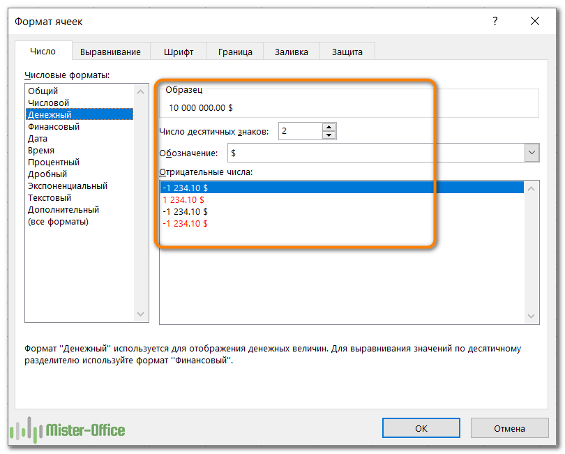
Денежный формат позволяет настроить следующие три параметра:
- Количество отображаемых десятичных знаков,
- Используемый символ валюты,
- Как будут выглядеть отрицательные числа.
Финансовый формат позволяет настроить только первые 2 параметра из перечисленных выше.

Разница между ними также заключается в следующем:
- Денежный помещает символ валюты непосредственно перед первой цифрой.
- В финансовом выравнивается символ валюты слева и значения справа, нули отображаются как прочерк.
Другие особенности этих двух похожих форматов мы подробно рассмотрели в этой статье.
Дата и время.
Microsoft Excel предоставляет множество предустановленных форматов даты и времени для разных языков:

Дополнительные сведения и подробные инструкции о том, как создать собственное представление даты и времени в Excel, см. в следующих разделах: Формат даты в Excel.
Процент.
Как легко догадаться, он отображает значение со знаком процента. Единственный параметр, который здесь можно изменить, – это количество десятичных знаков.
Чтобы быстро применить процентный формат без десятичных знаков, используйте комбинацию клавиш Ctrl + Shift +% .
Дополнительные сведения см. в разделе Как отображать проценты в Excel .
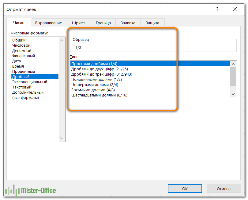
Дробь.
Здесь вам нужно выбирать из нескольких вариантов представления дроби:
Экспоненциальный формат
Экспоненциальный (научный) формат представляет собой компактный способ отображения очень больших или очень малых чисел. Его обычно используют математики, инженеры и ученые.
Например, вместо 0,0000000012 вы можете написать 1,2 x 10 -9. И если вы примените его к числу 0,0000000012, то получите 1,2E-09.
Единственный параметр, который вы можете здесь установить, – это количество десятичных знаков:
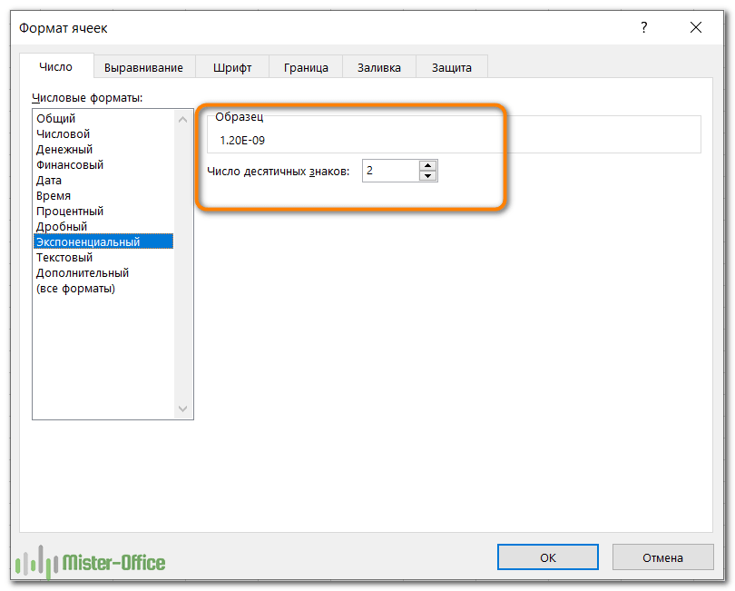
Чтобы быстро применить его с двумя знаками после запятой по умолчанию, нажмите на клавиатуре Ctrl + Shift + ^ .
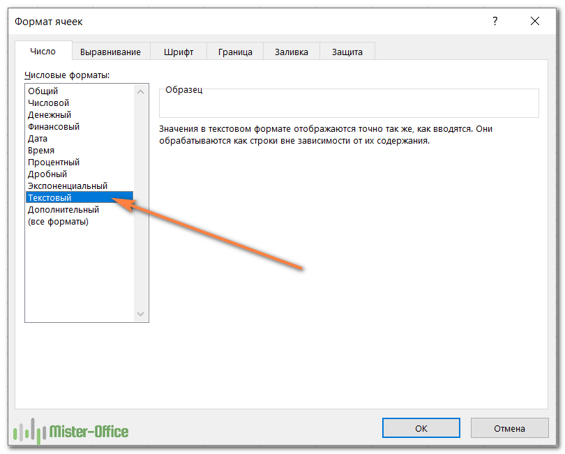
Текст.
Если ячейка отформатирована как текст, Excel будет рассматривать её содержимое как текстовую строку, даже если там записаны число или дата. По умолчанию текстовое представление выравнивает значения по левому краю.
Помните, что текстовый формат, применяемый к числам или датам, не позволяет использовать их в математических функциях и вычислениях Excel. Числовые значения, отформатированные как текст, выделяются маленьким зеленым треугольником в верхнем левом углу ячейки. Этот треугольник показывает, что в этой позиции что-то не так.
И если ваша, казалось бы, правильная формула Excel не работает или возвращает неправильный результат, то первое, что нужно проверить, – имеются ли числа, отформатированные как текст.
Чтобы исправить текстовые числа, недостаточно поменять формат на «Общий» или «Число». Самый простой способ преобразовать текст в число – выбрать проблемные позиции мышкой, затем щелкнуть появившийся треугольник, и выбрать опцию «Преобразовать в число» во всплывающем меню. Некоторые другие методы описаны в статье Как преобразовать цифры в текстовом формате в числа.
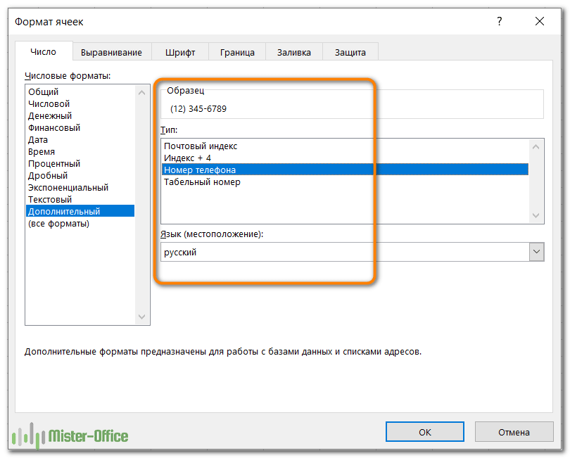
Специальный формат
Позволяет отображать числа в виде, обычном для почтовых индексов, номеров телефонов и табельных номеров:
Пользовательский формат
Если ни один из встроенных форматов не отображает данные так, как вы хотите, вы можете создать своё собственное представление для чисел, дат и времени. Вы сможете сделать это, изменив один из предопределенных форматов, близкий к желаемому результату, или же используя специальные символы форматирования в ваших собственных выражениях.
В следующей статье мы предоставим подробные инструкции и примеры для создания пользовательского числового формата в Excel.
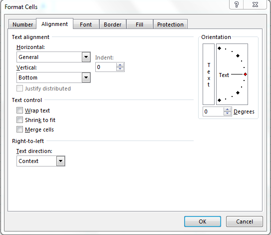
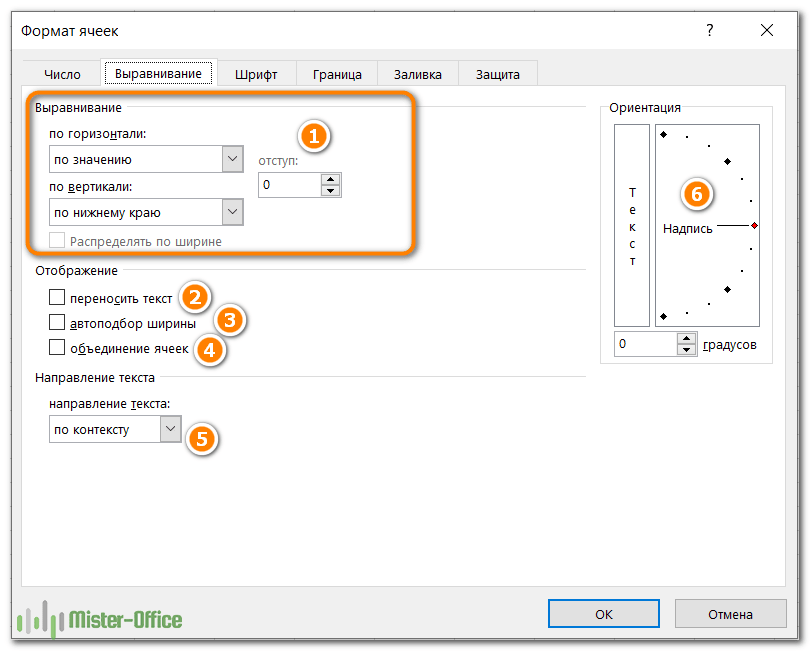
Вкладка «Выравнивание» — изменение выравнивания, положения и направления
Как следует из названия, эта вкладка позволяет изменять выравнивание текста. Кроме того, тут имеется ряд других опций, в том числе:
- Выровнять содержимое по горизонтали, вертикали или по центру. Кроме того, вы можете центрировать значение по выделению (отличная альтернатива слиянию ячеек!). Или делать отступ от любого края.
- Разбить текст на несколько строк в зависимости от ширины столбца и содержимого.
- Сжать по размеру — этот параметр автоматически уменьшает видимый размер шрифта, чтобы все данные помещались в столбце без переноса. Реальный установленный размер шрифта не изменяется.
- Объединить две или более ячеек в одну.
- Изменить направление текста. Значение по умолчанию — Контекст, но вы можете изменить его на Справа налево или Слева направо.
- Измените ориентацию текста. При вводе положительного числа в поле «Градусы» содержимое поворачивается из нижнего левого угла в верхний правый, а при отрицательном градусе выполняется поворот из верхнего левого угла в нижний правый. Этот параметр может быть недоступен, если ранее были выбраны другие параметры выравнивания.
На скриншоте показаны настройки вкладки «Выравнивание» по умолчанию:
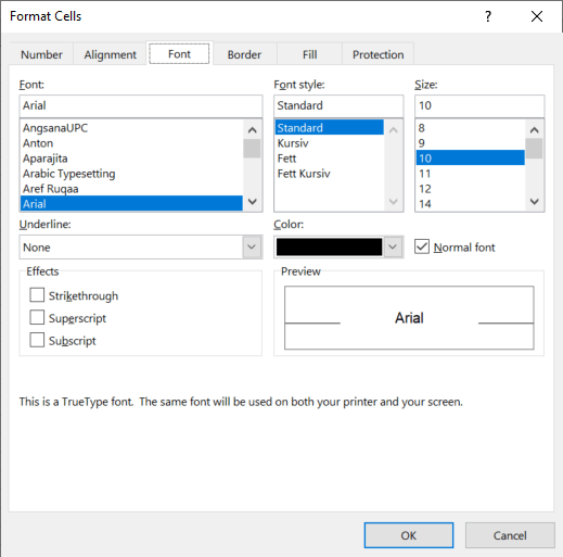
Вкладка «Шрифт» — изменение типа, цвета и стиля шрифта
Используйте её, чтобы изменить тип, цвет, размер, стиль, эффекты и другие элементы шрифта:

Думаю, здесь всё интуитивно понятно – всё как в текстовом редакторе.
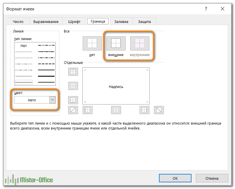
Вкладка «Граница» — создание границ ячеек разных стилей.
Используйте её, чтобы создать рамку вокруг выбранных ячеек в цвете и стиле по вашему выбору. Если вы не хотите удалять существующую границу, выберите «Нет».
Совет. Чтобы скрыть линии сетки в определенном диапазоне ячеек, вы можете применить белые границы (внешние и внутренние) к выбранным позициям, как показано на скриншоте ниже:
Вкладка «Заливка» — изменение цвета фона.
Вы можете закрашивать ячейки различными цветами, узорами, применять специальные эффекты заливки.

Вкладка Защита — заблокировать и скрыть ячейки
Используйте параметры защиты, чтобы заблокировать или скрыть определенные ячейки при защите рабочего листа.
Как настроить текст?
Разберем несколько способов того, как можно настроить текст, чтобы сделать таблицы с данными максимально читаемыми.
Как изменить шрифт.
Разберем несколько способов изменения шрифта:
- Способ первый. Выделяем ячейку, переходим в раздел «Главная» и выбираем элемент «Шрифт». Открывается список, в котором каждый пользователь сможет подобрать для себя подходящий шрифт.

- Способ второй. Выделяем ячейку, жмем на ней правой кнопкой мыши. Отображается контекстное меню, а рядом с ним небольшое окошко, позволяющее установить шрифт.
- Способ третий. При помощи комбинации клавиш Ctrl+1 вызываем уже знакомое нам окно. В нём выбираем раздел «Шрифт» и проводим все необходимые настройки. Про это мы уже рассказывали чуть выше.
Выбираем способы начертания.
Полужирные, курсивные и подчеркнутые начертания используются для выделения важной информации в таблицах. Чтобы изменить начертание всей ячейки, нужно нажать на нее левой кнопкой мыши. Для изменения только части ячейки нужно два раза кликнуть по ней, а затем отдельно выделить желаемую часть текста, с которой и будем работать. После выделения изменяем начертание одним из следующих методов:
- При помощи комбинации клавиш:
- Ctrl+B – полужирное;
- Ctrl+I – курсивное;
- Ctrl+U – подчеркнутое;
- Ctrl+5 – перечеркнутое;
- Ctrl+= – подстрочное;
- Ctrl+Shift++ – надстрочный.
- При помощи инструментов, находящихся в разделе «Шрифт» вкладки «Главная».
- Используя окошко «Формат ячеек». Здесь можно выставить нужные настройки в разделах «Видоизменение» и «Начертание» (подробнее см. выше)
Выравнивание текста.
Способ выравнивания текста можно установить следующими методами:
- Заходим в раздел «Выравнивание» вкладки «Главная». Здесь при помощи иконок можно установить способ выравнивания данных.
- В окошке «Формат ячеек» переходим в соответствующий раздел. Здесь тоже можно выбрать все нужные опции.
Параметры форматирования ячеек на ленте.
Как вы только что убедились, диалоговое окно «Форматирование ячеек» предоставляет большое количество возможностей. Для нашего удобства на ленте также доступны наиболее часто используемые инструменты.
Чтобы быстро применить один из форматов Excel с настройками по умолчанию, сделайте следующее:
- Выделите ячейку или диапазон, вид которых вы хотите изменить.
- Щелкните маленькую стрелку рядом с полем Формат числа на вкладке Главная в группе Число и выберите нужный вам:
Параметры финансового формата на ленте.
Группа Число предоставляет некоторые из наиболее часто используемых параметров для отображения финансовой информации:
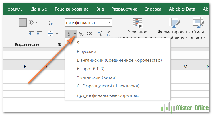
- Чтобы применить числовой формат с символом валюты по умолчанию, выберите ячейку и нажмите значок со знаком $.
- Чтобы выбрать другой символ валюты, щелкните стрелку рядом со значком доллара и выберите нужную валюту из списка. Если вы хотите использовать какой-либо другой символ валюты, нажмите «Другие финансовые форматы» в конце списка, откроется диалоговое окно с дополнительными параметрами.
- Чтобы использовать разделитель тысяч, нажмите значок с нулями 000.
- Чтобы отобразить больше или меньше десятичных знаков, используйте иконки «Увеличить разрядность» или «Уменьшить разрядность» соответственно. Это можно применить для финансового формата, а также для числового, процентного и денежного.
Другие параметры форматирования на ленте.
На вкладке «Главная» имеется еще несколько параметров – изменение границ ячеек, цветов заливки и шрифта, выравнивания. Например, чтобы быстро добавить границы, щелкните стрелку рядом с кнопкой Границы в группе Шрифт и выберите желаемый макет, цвет и стиль:

Вновь видим, что одно и тоже можно сделать несколькими способами – ведь про оформление границ мы уже говорили выше.
Быстрые клавиши для изменения формата данных в Excel.
Если вы внимательно изучили предыдущие разделы этого руководства, вы уже знаете большинство сочетаний клавиш форматирования Excel. В таблице ниже мы их обобщим:
| Клавиши | Применяемый формат |
| Ctrl + Shift + ~ | Общий числовой формат |
| Ctrl + Shift +! | Число с разделителем тысяч, двумя десятичными разрядами и знаком минус (-) для отрицательных значений |
| Ctrl + Shift + $ | Валюта с двумя десятичными знаками и отрицательными числами, отображаемыми в скобках. |
| Ctrl + Shift +% | Проценты без десятичных знаков |
| Ctrl + Shift + ^ | Экспоненциальный (научный) с двумя десятичными знаками |
| Ctrl + Shift + # | Дата (дд-ммм-гг) |
| Ctrl + Shift + @ | Время (чч: мм: сс) |
Почему не работает форматирование?
Если после изменения одного из числовых форматов Excel в ячейке появляется несколько хеш-символов (######), то обычно это происходит по одной из следующих причин:
- Ячейка недостаточно широка для отображения данных в выбранном представлении. Чтобы исправить это, чаще всего всё, что вам нужно сделать — это увеличить ширину столбца, перетащив мышкой его правую границу. Или же просто дважды щелкните правую границу, чтобы автоматически изменить его размер, который сам подстроится под наибольшее значение в столбце.
- Ячейка содержит отрицательную дату или дату вне поддерживаемого диапазона дат (с 01.01.1900 по 31.12.9999).
Чтобы различать эти два случая, наведите указатель мыши на знаки решетки. Если там какое-то допустимое значение, которое слишком велико, чтобы поместиться в ячейку, Excel отобразит всплывающую подсказку с реальным значением. Если указана неверная дата, вы получите уведомление о проблеме.
И второй случай, который достаточно часто встречается. Excel не меняет формат ячейки. Точнее, он меняет, но представление данных остаётся прежним.
Вы пытаетесь изменить представление даты, но ничего не происходит. Причина в том, что у вас дата записана в виде текста. Если вы будете пытаться формат для чисел применить к тексту, то ничего не произойдет. Как превратить текст в настоящую дату — читайте здесь.
Как избежать автоматического форматирования данных в Excel?
Excel — полезная программа, когда у вас есть стандартные задачи и стандартные данные. Если вы захотите пойти своим нестандартным путем, может появиться некоторое разочарование. Особенно, когда у нас большие наборы данных. Я столкнулся с одной из таких проблем, когда работал с задачами наших клиентов в Excel.
Удивительно, но это оказалось довольно распространенной проблемой: мы вводим цифры вместе с тире или косой чертой, и Excel тут же решает, что это дата. И сразу изменяет формат, не спрашивая вас.
Итак, если вы хотите найти ответ на вопрос: «Можно ли отменить автоматическое форматирование?», то ответ, к сожалению, «Нет». Но есть несколько способов справиться с таким навязчивым поведением программы.
Предварительное форматирование ячеек перед вводом данных.
Это действительно довольно простое решение, если вы только вводите данные в свою таблицу. Самый быстрый способ — следующий:
- Выберите диапазон, в котором у вас будут особые данные. Это может быть столбец или диапазон. Вы даже можете выбрать весь рабочий лист (нажмите Ctrl + A, чтобы сделать это сразу)
- Щелкните правой кнопкой мыши выбранное и используйте пункт «Форматировать ячейки…». Или просто нажмите
Ctrl + 1. - Выберите текст в списке категорий на вкладке «Число».
- Нажмите ОК
Это то, что нужно: всё, что вы вводите в этот столбец или рабочий лист, сохранит свой исходный вид: будь то 1–4 или мар-5. Оно рассматривается как текст, выровнено по левому краю, вот и все.
Совет: вы можете автоматизировать эту задачу как в масштабе листа, так и в масштабе ячейки. Некоторые профи на форумах предлагают создать шаблон рабочего листа, который можно использовать в любое время:
- Отформатируйте лист как текст, следуя шагам выше;
- Сохранить как… — тип файла шаблона Excel. Теперь каждый раз, когда вам нужен рабочий лист в текстовом формате, вы можете использовать его в своих личных шаблонах и создать из него новый лист.
Если вам нужны ячейки с текстовым форматированием — создайте собственный стиль ячеек в разделе «Стили» на вкладке «Главная». Создав один раз, вы можете быстро применить его к выбранному диапазону ячеек и ввести данные.
Ввод данных в виде текста.
Другой способ запретить Excel автоматически менять формат ячеек — ввести апостроф (‘) перед вводимым вами значением. По сути, эта операция делает то же самое – жёстко определяет ваши данные как текст.
Копирование форматов в Excel.
После того, как вы приложили много усилий для расчета таблицы, вы обычно хотите добавить несколько штрихов, чтобы она выглядела красиво и презентабельно. Независимо от того, создаете ли вы отчет для своего головного офиса или сводный рабочий лист для руководства, правильное оформление — это то, что выделяет важные данные и более эффективно передает соответствующую информацию.
К счастью, в Microsoft Excel есть удивительно простой способ скопировать форматирование, которое часто упускают из виду. Как вы, наверное, догадались, я говорю об инструменте «Формат по образцу», который позволяет очень легко применить параметры отображения одной ячейки к другой.
Далее в этом руководстве вы найдете наиболее эффективные способы его использования и изучите несколько других методов для копирования форматирования в ваших таблицах.
Формат по образцу.
Он работает, копируя офорление одной ячейки и применяя его к другим.
Всего за пару щелчков мышью вы сможете изменить большую часть параметров внешнего вида, в том числе:
- Вид числа (общий, процентный, денежный и т. д.),
- Начертание, размер и цвет шрифта,
- Характеристики шрифта, такие как полужирный, курсив и подчеркивание,
- Цвет заливки (цвет фона),
- Выравнивание текста, направление и ориентация,
- Границы ячеек.
Во всех версиях Excel кнопка вызова этой функции находится на вкладке «Главная» в группе «Буфер обмена», рядом с кнопкой «Вставить» :

Чтобы скопировать форматирование ячеек, сделайте следующее:
- Выделите ячейку с тем оформлением, которое вы хотите скопировать.
- На вкладке «Главная» в группе «Буфер обмена» нажмите кнопку «Формат по образцу». Указатель мышки превратится в кисть.
- Кликните мышкой туда, где вы хотите применить это.
Готово! Целевая ячейка теперь выглядит по-новому.
![]()
Если вам нужно изменить оформление более чем одной ячейки, нажатие на каждую из них по отдельности будет утомительным и трудоемким. Следующие советы помогут ускорить процесс.
1. Как скопировать форматирование в диапазон ячеек.
Чтобы скопировать в несколько соседних ячеек, выберите образец с желаемыми параметрами, нажмите кнопку «Формат по образцу», а затем протащите курсор кисти по ячейкам, которые вы хотите оформить.
2. Как скопировать формат в несмежные ячейки.
Чтобы скопировать в несмежные ячейки, дважды нажмите кнопку «Формат по образцу», а не один раз. Это «заблокирует» кисть, и скопированные параметры будут применяться ко всем позициям и диапазонам, которые вы щелкаете кисточкой, пока вы не нажмете клавишу Esc или же еще раз эту кнопку.
3. Как скопировать форматирование одного столбца в другой столбец построчно.
Чтобы быстро скопировать внешний вид всего столбца, выберите его заголовок, щелкните на кнопку с кисточкой, а затем кликните заголовок целевого столбца.
Новое оформление применяется к целевому столбцу построчно, включая ширину.
Таким же образом вы можете скопировать формат строки. Для этого щелкните заголовок строки-образца, нажмите на кисточку, а затем щелкните заголовок целевой строки.
Думаю, вы согласитесь, что это делает копирование формата настолько простым, насколько это возможно. Однако, как это часто бывает с Microsoft Excel, есть несколько способов выполнить любое действие.
Вот еще два метода.
Использование маркера заполнения.
Мы часто используем маркер заполнения для копирования формул или автоматического заполнения ячеек данными. Но знаете ли вы, что он также может копировать форматы Excel всего за несколько кликов? Вот как:
- Установите вид первой ячейки так, как это необходимо.
- Выберите эту правильно отформатированную ячейку и наведите указатель мыши на маркер заполнения (небольшой квадрат в правом нижнем углу). При этом курсор изменится с белого креста выбора на черный крестик.
- Удерживайте и перетащите маркер над ячейками, к которым вы хотите применить форматирование.
Это также скопирует значение первой из них в остальные. Но не беспокойтесь об этом, мы отменим это на следующем шаге. - Отпустите маркер заполнения, щелкните раскрывающееся меню и выберите Заполнить только форматы:
Это оно! Значения ячеек возвращаются к исходным, и желаемый внешний вид применяется к нужным ячейкам в столбце.
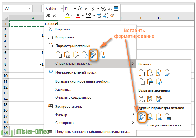
Специальная вставка.
Предыдущие два инструмента отлично работают с небольшими областями данных. Но как скопировать формат определенной ячейки на весь столбец или строку, чтобы он применялся абсолютно ко всем позициям, включая пустые? Решение заключается в использовании опции «Форматы» в инструменте «Специальная вставка».
- Выберите ячейку с желаемым форматом и нажмите
Ctrl + C, чтобы копировать её полностью в буфер обмена. - Выделите весь столбец или строку, которую хотите отформатировать, щелкнув ее заголовок.
- Кликните на выделенном правой кнопкой мыши и выберите «Специальная вставка».
- В появившемся диалоговом окне нажмите «Форматы», а затем — « ОК» .

Либо выберите параметр «Форматирование» в том же всплывающем меню:
«Найти и выделить».
Инструмент «Найти и выделить» может искать не только значения, но и форматы. С его помощью также можно быстро менять вид вашей таблицы. Особенно это хорошо тогда, когда ячейки, которые нужно изменить, разбросаны по всему рабочему листу и вручную выделить их все будет довольно проблематично.
Предположим, в нашей таблице нужно заменить финансовый формат на денежный. И руками кликать кисточкой на каждую клетку будет очень долго. Да ещё и обязательно что-то пропустишь…
Итак, давайте рассмотрим небольшой пример. У нас есть образец в A1. Точно таким же образом мы хотим оформить все ячейки с форматом «Общий».
На ленте активируем инструмент «Найти и выделить» – «Заменить». Не вводим никаких значений для поиска, а используем кнопку «Формат» – «Выбрать формат из ячейки»
На скриншоте ниже вы можете наблюдать весь этот процесс.
После выбора исходного формата, в поле «Заменить на» можно выбрать новый, которым можно заменить исходный. Как видите, процедура в целом та же, что и при замене одних значений другими.
Клавиши для копирования форматирования в Excel.
К сожалению, Microsoft Excel не предоставляет ни одной комбинации клавиш, которую можно было бы использовать для копирования форматов ячеек. Однако это можно сделать с помощью последовательности команд. Итак, если вы предпочитаете большую часть времени работать с клавиатуры, вы можете скопировать формат в Excel одним из следующих способов.
Клавиши для формата по образцу.
Вместо того, чтобы нажимать кнопку на ленте, сделайте следующее:
- Выделите ячейку, содержащую нужный формат.
- Нажмите Alt, H, F, P.
- Щелкните цель, к которой вы хотите применить форматирование.
Обратите внимание, что эти клавиши следует нажимать одну за другой, а не все сразу:
- Alt активирует сочетания клавиш для команд ленты.
- H выбирает вкладку «Главная» на ленте.
- Нажатие F а затем — P, активирует кисть.
Клавиши специального форматирования.
Еще один быстрый способ скопировать формат в Excel — использовать сочетание клавиш для Специальной вставки > Форматы :
- Выберите ячейку, которую используем как образец.
- Используйте
Ctrl + Cчтобы скопировать ее в буфер обмена. - Выберите, где будем менять оформление.
- Нажмите
Shift + F10, S, R, а затем щелкните Войти.
Если кто-то все еще использует Excel 2007, нажмите Shift + F10, S, T, ввод.
Эта последовательность клавиш выполняет следующее:
- Shift + F10 отображает контекстное меню.
- комбинация Shift + S выбирает команду «Специальная вставка».
- Shift + R выбирает для вставки только форматирование.
Это самые быстрые способы скопировать форматирование в Excel.
Работа со стилями форматирования ячеек Excel
Использование стилей позволяет значительно ускорить процесс оформления таблицы и придать ей красивый внешний вид.

Основная цель использования стилей – автоматизация работы с данными. Используя стиль, можно быстро оформить выделенный диапазон. Для вас уже создано большое количество интегрированных готовых стилей. Как ими пользоваться – разберём пошагово:
- Выделяем необходимую ячейку или диапазон.
- Переходим на вкладку «Главная», находим на ленте раздел «Стили ячеек».
- Нажимаем, и на экране появляется библиотека готовых стилей.
- Кликаем на понравившийся стиль. Стиль применился к ячейке. Если просто навести мышку на предлагаемый стиль, но не нажимать на него, то можно предварительно посмотреть прямо на рабочем листе, как он будет выглядеть.
Как создать или изменить стиль?
Часто пользователям недостаточно готовых стилей, и они прибегают к разработке собственных. Сделать свой уникальный стиль можно следующим образом:
- Выделяем любую ячейку и устанавливаем в ней все необходимые параметры. Это будет наш образец для создания нового стиля.
- Переходим в раздел «Главная» в блок «Стили ячеек». Кликаем «Создать …». Открылось окошко под названием «Стиль».
- Вводим любое имя.
- Выставляем все необходимые параметры, которые вы желаете включить.
- Кликаем «ОК».
- Теперь в библиотеку стилей добавился ваш новый уникальный, который можно использовать в этом документе.

Готовые стили, располагающиеся в библиотеке, можно самостоятельно изменять:
- Переходим в раздел «Стили ячеек».
- Жмем правой кнопкой мыши по стилю, который желаем отредактировать, и кликаем «Изменить».
- В открывшемся окошке кликаем «Формат», далее – «Формат ячеек» настраиваем уже знакомые нам опции. После проведения всех манипуляций кликаем «ОК».
- Снова нажимаем «ОК», чтобы закрыть. Редактирование завершено.
Перенос стилей в другую книгу.
Вот последовательность действий:
- Отрываем документ, в котором находятся созданные стили.
- Также открываем другой документ, в который желаем их перенести.
- В исходном документе переходим во вкладку «Главная» и находим раздел «Стили».
- Кликаем «Объединить». Появилось окошко «Объединение».
- В нем видим список всех открытых документов. Выбираем тот из них, в который хотим перенести созданный стиль и кликаем кнопку «ОК». Готово!
Итак, теперь вы владеете основными навыками, чтобы настроить формат ячеек в Excel. Но если вы случайно установили неудачный вид – это не проблема! Наша следующая статья научит вас, как его очистить 
Благодарю вас за чтение и надеюсь вновь увидеть вас в нашем блоге!
 Формат времени в Excel — Вы узнаете об особенностях формата времени Excel, как записать его в часах, минутах или секундах, как перевести в число или текст, а также о том, как добавить время с помощью…
  Как сделать пользовательский числовой формат в Excel — В этом руководстве объясняются основы форматирования чисел в Excel и предоставляется подробное руководство по созданию настраиваемого пользователем формата. Вы узнаете, как отображать нужное количество десятичных знаков, изменять выравнивание или цвет шрифта,…
  8 способов разделить ячейку Excel на две или несколько — Как разделить ячейку в Excel? С помощью функции «Текст по столбцам», мгновенного заполнения, формул или вставив в нее фигуру. В этом руководстве описаны все варианты, которые помогут вам выбрать технику, наиболее подходящую…
Does this sound familiar? You work on an Excel sheet and are almost done with it. Now, you just want to “brush it up” a bit. But: It seems that the formatting takes even longer than working on the calculations. In this article we look at techniques to apply a format with as few clicks as possible. Let’s start saving time now!
Method 1: How to format cells manually
Potential time saving: ![]()
![]()
![]()
![]()
![]()
Well, probably you are not here for learning it the long, inconvenient way. But anyway, I quickly summarize how to apply a format the “traditional” way in Excel.
Actually, there are several way to change font, number formatting, colors, borders. The first one would be via the ribbon:
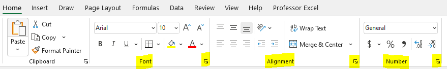
On the Home ribbon, you can find the quick settings of font style, colors, borders and so in the “Font” group. Next to it, you can see further settings in the “Alignment” group and the “Number” group. Everything, no need to elaborate that in detail.
One comment: the small arrows in the corners (also highlighted yellow), lead to the Format cells window. It contains more detailed formatting options. Alternatively, you can just press Ctrl + 1 on the keyboard to open that window.
Method 2: Shortcut formatting with the format painter
Potential time saving: ![]()
![]()
![]()
![]()
![]()
Once you have perfectly formatted a cell (for example with the method 1 above). With the Format Painter, you can easily transfer this formatting to a different cell.
- Select the original cells.
- Click on the Format Painter on the Home ribbon.
- Click on the unformatted cell to apply the format.
You want to apply this cell layout to multiple cells? Double click on the format painter and the you can click on all desired cells until you press Esc or click on the Format Painter button again.
Also: It works for whole ranges of cells. You can just select multiple cells and press on the Format Painter button.

Recommendation: This could be a great button for the Quick Access Toolbar. I have added it to my Quick Access Toolbar – in all Office programs at the same position. Now, when I press the Alt button and afterwards 4 (because it is in the forth position in my Quick Access Toolbar), I can quickly use it without the mouse.
Method 3: Apply cell styles to save a lot of time
Potential time saving: ![]()
![]()
![]()
![]()
![]()
Now, we get increasingly faster with formatting. Our next advice is to use the built-in cell styles.
Cell styles are a great way to apply layout settings to single cells are cell ranges. And later, you can easily change the format within the cell style definition.
Here is, how it works:
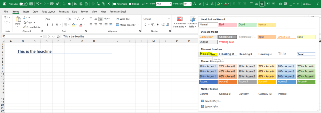
- Select one or multiple cells.
- Click on your desired cell style. It’s located on the Home ribbon in the Styles section.
Changing a cell style is quite simple, but requires some clicks through the menues.
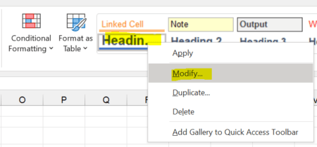
- Right-click on the style you want to change.
- Then, click on Modify.
- Now, you can click on “Format” to change the settings in detail.
The changes will be applied to all cells that use this particular style.
Disadvantages:
- When you copy worksheets several times from different files, cell styles might accumulated. I have noticed that especially for some Excel exports, for example from SAP.
- If you change a cell style, it only applies to the current Excel workbook. When you create a new Excel file, you have to do the same changes again.
Method 4: Use Office themes
Potential time saving: ![]()
![]()
![]()
![]()
![]()
This method works best when you already have a “clean” formatting in your Excel file. For example, if you have consequently used the cell styles in method 3 above.
But nonetheless, it’s often a worth a try: Create your own Office theme. This can save a lot of time when it comes to colors and fonts. The advantage: You can save a theme and use it throughout the Office suite. That way, you can transfer your corporate colors to all your documents.
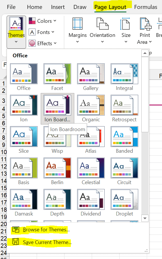
How it works? Quit simple:
- Go to the Page Layout ribbon.
- Click on the theme that is already close to your desired layout.
- Modify colors and fonts with the buttons right next to the Themes button.
- Click on “Save Current Theme”.
Next time you want to use this theme, just click on “Browse for theme” and select it on your hard drive.
Do you want to boost your productivity in Excel?
Get the Professor Excel ribbon!

Add more than 120 great features to Excel!
Method 5: Use Professor Excel Tools to use your individual formatting – with just one click
Potential time saving: ![]()
![]()
![]()
![]()
![]()
This is probably the feature I use most often of the Excel add-in “Professor Excel Tools“. It’s fair to say that I have saved days, maybe even weeks of work just with these two buttons.
- Just select the cells to format.
- Click on either the headline or content / body button.
As you can see, it’s very fast, right?
The good thing about this method: You just define it once – and you can apply the formatting to any workbook.
Defining your favorite formats is also very easy:
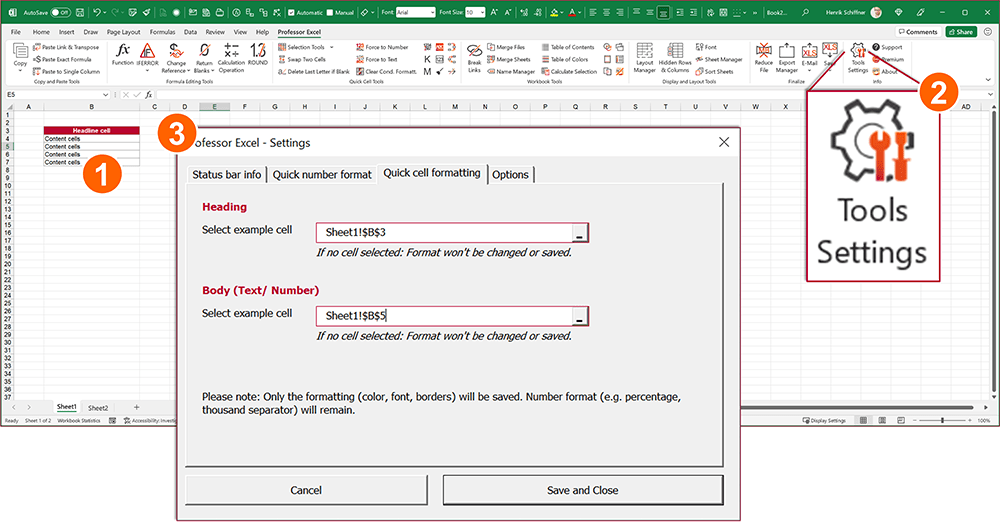
- Apply your favorite heading or content / body layout to a cell.
- Go to the Tools Settings (on the right side of the Professor Excel ribbon).
- On the “Quick cell formatting” tab, select your pre-formatted example cells for heading and body. Click on Save and Close to save the formatting.

This function is included in our Excel Add-In ‘Professor Excel Tools’
(No sign-up, download starts directly)
Image by garageband from Pixabay
Содержание
- Основные виды форматирования и их изменение
- Способ 1: контекстное меню
- Способ 2: блок инструментов «Число» на ленте
- Способ 3: блок инструментов «Ячейки»
- Способ 4: горячие клавиши
- Вопросы и ответы

Формат ячейки в программе Эксель задает не просто внешний вид отображения данных, но и указывает самой программе, как именно их следует обрабатывать: как текст, как числа, как дату и т.д. Поэтому очень важно правильно установить данную характеристику диапазона, в который будут вноситься данные. В обратном случае, все вычисления будут просто некорректными. Давайте выясним, как изменить формат ячеек в Microsoft Excel.
Урок: Форматирование текста в Microsoft Word
Основные виды форматирования и их изменение
Сразу определим, какие форматы ячеек существуют. Программа предлагает выбрать один из следующих основных видов форматирования:
- Общий;
- Денежный;
- Числовой;
- Финансовый;
- Текстовый;
- Дата;
- Время;
- Дробный;
- Процентный;
- Дополнительный.
Кроме того, существует разделение на более мелкие структурные единицы вышеуказанных вариантов. Например, форматы даты и времени имеют несколько подвидов (ДД.ММ.ГГ., ДД.месяц.ГГ, ДД.М, Ч.ММ PM, ЧЧ.ММ и др.).
Изменить форматирование ячеек в Excel можно сразу несколькими способами. О них мы подробно поговорим ниже.
Способ 1: контекстное меню
Самый популярный способ изменения форматов диапазона данных – это использование контекстного меню.
- Выделяем ячейки, которые нужно соответствующим образом отформатировать. Выполняем клик правой кнопкой мыши. Вследствие этого открывается контекстный список действий. Нужно остановить выбор на пункте «Формат ячеек…».
- Активируется окно форматирования. Выполняем переход во вкладку «Число», если окно было открыто в другом месте. Именно в блоке параметров «Числовые форматы» находятся все те варианты изменения характеристик, о которых шел разговор выше. Выбираем пункт, который соответствует данным, находящимся в выбранном диапазоне. При необходимости в правой части окна определяем подвид данных. Жмем на кнопку «OK».
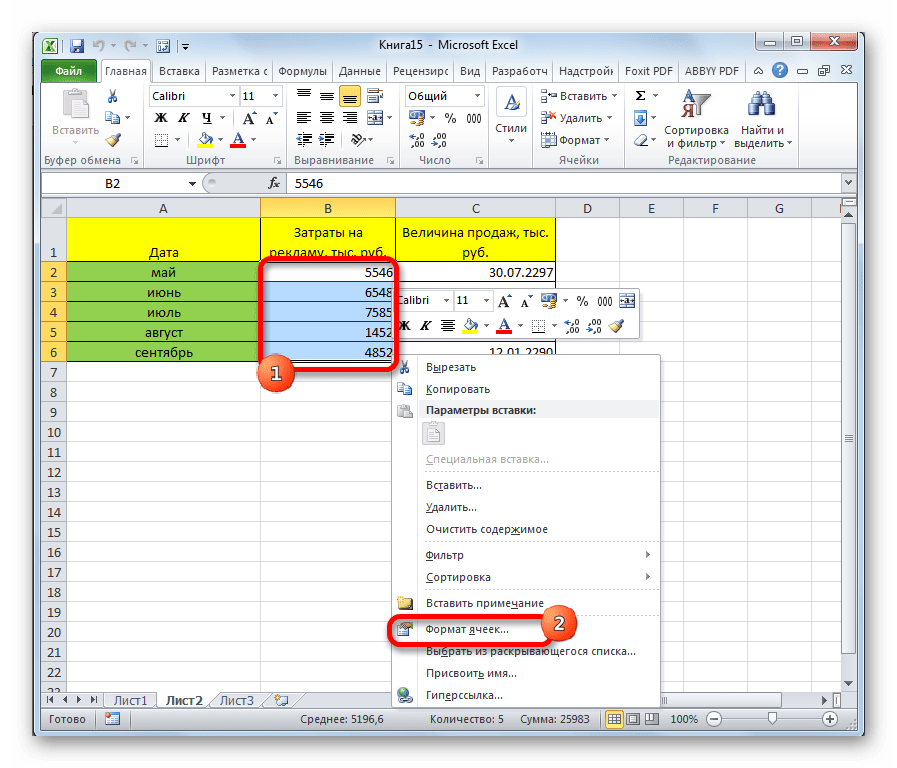
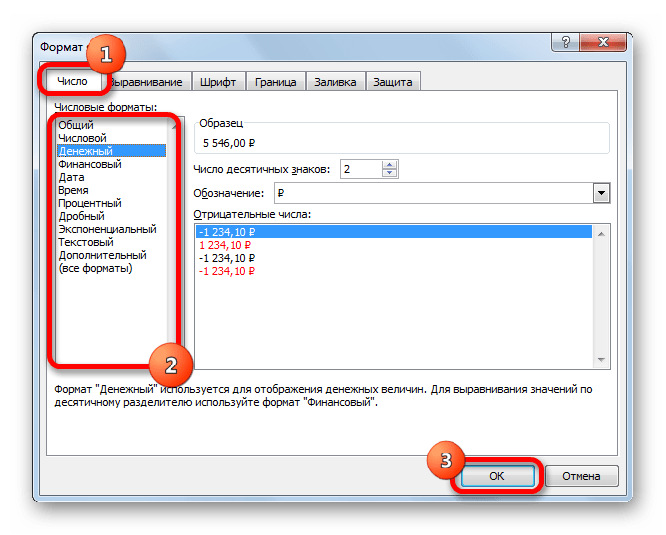
После этих действий формат ячеек изменен.
Способ 2: блок инструментов «Число» на ленте
Форматирование также можно изменить, используя инструменты, находящиеся на ленте. Этот способ выполняется даже быстрее предыдущего.
- Переходим во вкладку «Главная». При этом, нужно выделить соответствующие ячейки на листе, а в блоке настроек «Число» на ленте открыть поле выбора.
- Просто производим выбор нужного варианта. Диапазон сразу же после этого изменит своё форматирование.
- Но в указанном списке представлены только основные форматы. Если вы хотите более точно указать форматирование, то следует выбрать пункт «Другие числовые форматы».
- После данных действий, откроется окно форматирования диапазона, о котором уже шёл разговор выше. Пользователь может выбрать тут любой из основных или дополнительных форматов данных.
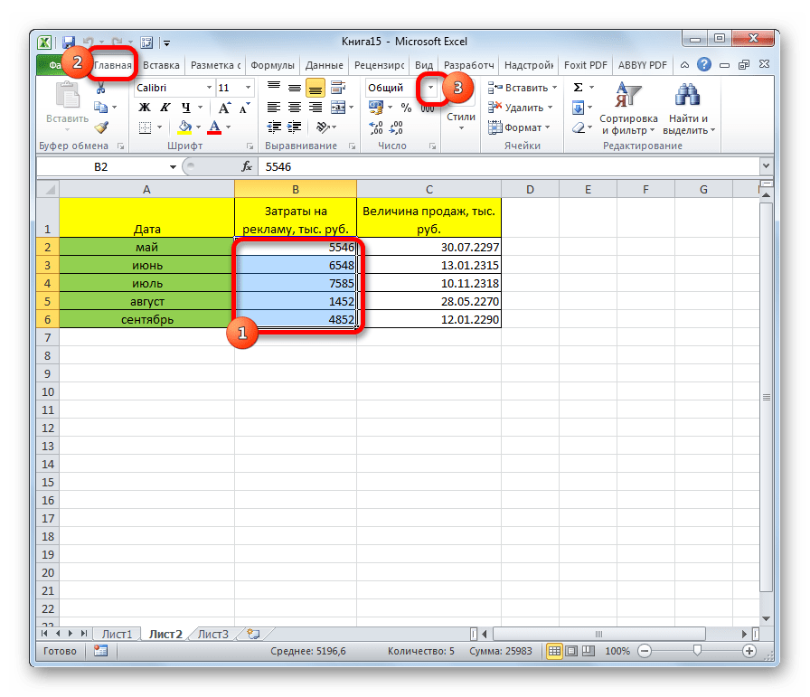
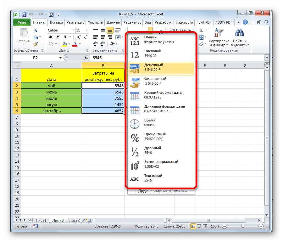
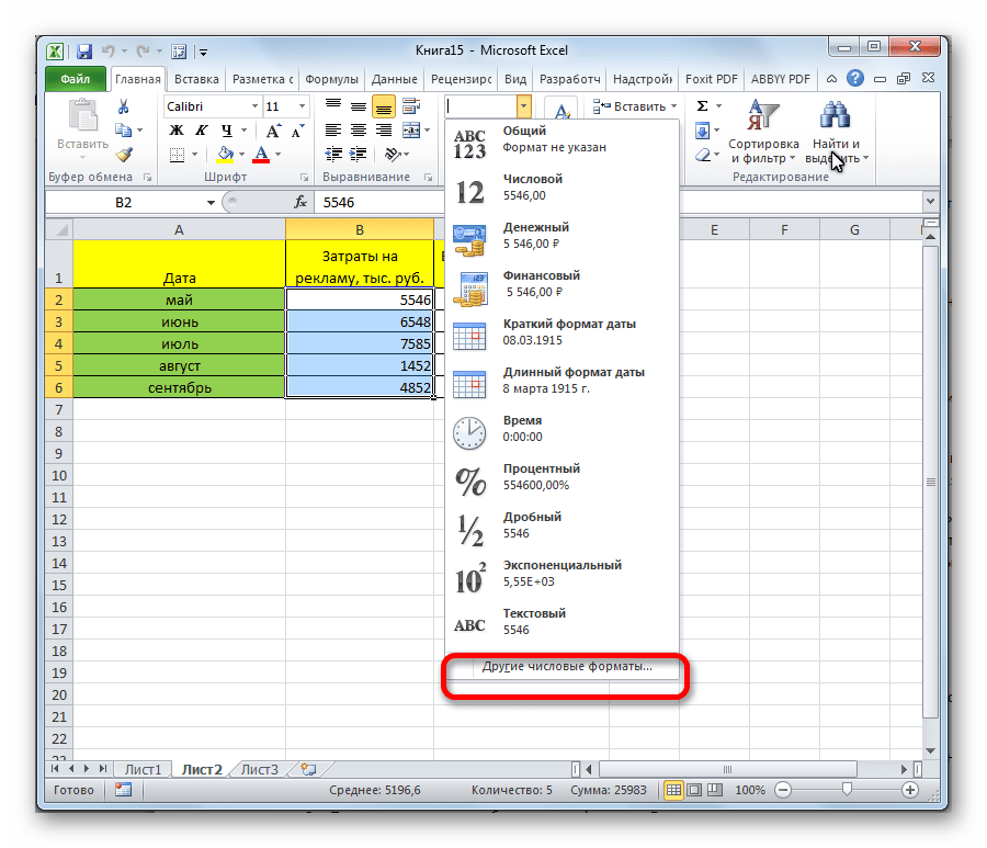
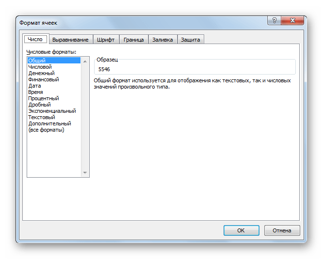

Способ 3: блок инструментов «Ячейки»
Ещё одним вариантом настройки данной характеристики диапазона является использования инструмента в блоке настроек «Ячейки».
- Выделяем диапазон на листе, который следует отформатировать. Располагаясь во вкладке «Главная», кликаем по значку «Формат», который находится в группе инструментов «Ячейки». В открывшемся списке действий выбираем пункт «Формат ячеек…».
- После этого активируется уже хорошо знакомое нам окно форматирования. Все дальнейшие действия точно такие же, как уже было описано выше.
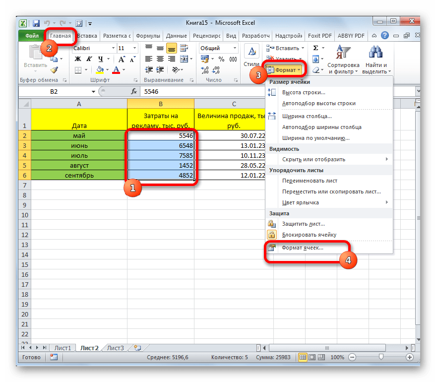
Способ 4: горячие клавиши
И наконец, окно форматирования диапазона можно вызвать при помощи так называемых горячих клавиш. Для этого нужно предварительно выделить изменяемую область на листе, а затем набрать на клавиатуре комбинацию Ctrl+1. После этого, откроется стандартное окно форматирования. Изменяем характеристики так же, как об этом было уже сказано выше.
Кроме того, отдельные комбинации горячих клавиш позволяют менять формат ячеек после выделения диапазона даже без вызова специального окна:
- Ctrl+Shift+- — общий формат;
- Ctrl+Shift+1 — числа с разделителем;
- Ctrl+Shift+2 — времени (часы.минуты);
- Ctrl+Shift+3 — даты (ДД.ММ.ГГ);
- Ctrl+Shift+4 – денежный;
- Ctrl+Shift+5 – процентный;
- Ctrl+Shift+6 — формат О.ООЕ+00.
Урок: Горячие клавиши в Экселе
Как видим, существует сразу несколько способов отформатировать области листа Excel. Эту процедуру можно совершить, воспользовавшись инструментами на ленте, вызовом окна форматирования или горячими клавишами. Каждый пользователь сам решает, какой вариант для него является наиболее удобным в решении конкретно поставленных задач, ведь в одних случаях достаточно применения общих форматов, а в других — требуется точное указание характеристик по подвидам.
Еще статьи по данной теме: