
Format numbers as dates or times
Excel for Microsoft 365 Excel for Microsoft 365 for Mac Excel for the web Excel 2021 Excel 2021 for Mac Excel 2019 Excel 2019 for Mac Excel 2016 Excel 2016 for Mac Excel 2013 Excel 2010 Excel 2007 Excel for Mac 2011 More…Less
When you type a date or time in a cell, it appears in a default date and time format. This default format is based on the regional date and time settings that are specified in Control Panel, and changes when you adjust those settings in Control Panel. You can display numbers in several other date and time formats, most of which are not affected by Control Panel settings.
In this article
-
Display numbers as dates or times
-
Create a custom date or time format
-
Tips for displaying dates or times
Display numbers as dates or times
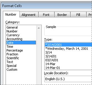
You can format dates and times as you type. For example, if you type 2/2 in a cell, Excel automatically interprets this as a date and displays 2-Feb in the cell. If this isn’t what you want—for example, if you would rather show February 2, 2009 or 2/2/09 in the cell—you can choose a different date format in the Format Cells dialog box, as explained in the following procedure. Similarly, if you type 9:30 a or 9:30 p in a cell, Excel will interpret this as a time and display 9:30 AM or 9:30 PM. Again, you can customize the way the time appears in the Format Cells dialog box.
-
On the Home tab, in the Number group, click the Dialog Box Launcher next to Number.

You can also press CTRL+1 to open the Format Cells dialog box.
-
In the Category list, click Date or Time.
-
In the Type list, click the date or time format that you want to use.
Note: Date and time formats that begin with an asterisk (*) respond to changes in regional date and time settings that are specified in Control Panel. Formats without an asterisk are not affected by Control Panel settings.
-
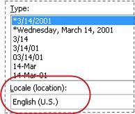
To display dates and times in the format of other languages, click the language setting that you want in the Locale (location) box.
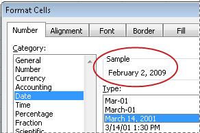
The number in the active cell of the selection on the worksheet appears in the Sample box so that you can preview the number formatting options that you selected.

Top of Page
Create a custom date or time format
-
On the Home tab, click the Dialog Box Launcher next to Number.
You can also press CTRL+1 to open the Format Cells dialog box.
-
In the Category box, click Date or Time, and then choose the number format that is closest in style to the one you want to create. (When creating custom number formats, it’s easier to start from an existing format than it is to start from scratch.)
-
In the Category box, click Custom. In the Type box, you should see the format code matching the date or time format you selected in the step 3. The built-in date or time format can’t be changed or deleted, so don’t worry about overwriting it.
-
In the Type box, make the necessary changes to the format. You can use any of the codes in the following tables:
Days, months, and years
|
To display |
Use this code |
|---|---|
|
Months as 1–12 |
m |
|
Months as 01–12 |
mm |
|
Months as Jan–Dec |
mmm |
|
Months as January–December |
mmmm |
|
Months as the first letter of the month |
mmmmm |
|
Days as 1–31 |
d |
|
Days as 01–31 |
dd |
|
Days as Sun–Sat |
ddd |
|
Days as Sunday–Saturday |
dddd |
|
Years as 00–99 |
yy |
|
Years as 1900–9999 |
yyyy |
If you use «m» immediately after the «h» or «hh» code or immediately before the «ss» code, Excel displays minutes instead of the month.
Hours, minutes, and seconds
|
To display |
Use this code |
|---|---|
|
Hours as 0–23 |
h |
|
Hours as 00–23 |
hh |
|
Minutes as 0–59 |
m |
|
Minutes as 00–59 |
mm |
|
Seconds as 0–59 |
s |
|
Seconds as 00–59 |
ss |
|
Hours as 4 AM |
h AM/PM |
|
Time as 4:36 PM |
h:mm AM/PM |
|
Time as 4:36:03 P |
h:mm:ss A/P |
|
Elapsed time in hours; for example, 25.02 |
[h]:mm |
|
Elapsed time in minutes; for example, 63:46 |
[mm]:ss |
|
Elapsed time in seconds |
[ss] |
|
Fractions of a second |
h:mm:ss.00 |
AM and PM If the format contains an AM or PM, the hour is based on the 12-hour clock, where «AM» or «A» indicates times from midnight until noon and «PM» or «P» indicates times from noon until midnight. Otherwise, the hour is based on the 24-hour clock. The «m» or «mm» code must appear immediately after the «h» or «hh» code or immediately before the «ss» code; otherwise, Excel displays the month instead of minutes.
Creating custom number formats can be tricky if you haven’t done it before. For more information about how to create custom number formats, see Create or delete a custom number format.
Top of Page
Tips for displaying dates or times
-
To quickly use the default date or time format, click the cell that contains the date or time, and then press CTRL+SHIFT+# or CTRL+SHIFT+@.
-
If a cell displays ##### after you apply date or time formatting to it, the cell probably isn’t wide enough to display the data. To expand the column width, double-click the right boundary of the column containing the cells. This automatically resizes the column to fit the number. You can also drag the right boundary until the columns are the size you want.
-
When you try to undo a date or time format by selecting General in the Category list, Excel displays a number code. When you enter a date or time again, Excel displays the default date or time format. To enter a specific date or time format, such as January 2010, you can format it as text by selecting Text in the Category list.
-
To quickly enter the current date in your worksheet, select any empty cell, and then press CTRL+; (semicolon), and then press ENTER, if necessary. To insert a date that will update to the current date each time you reopen a worksheet or recalculate a formula, type =TODAY() in an empty cell, and then press ENTER.
Need more help?
You can always ask an expert in the Excel Tech Community or get support in the Answers community.
Need more help?
Want more options?
Explore subscription benefits, browse training courses, learn how to secure your device, and more.
Communities help you ask and answer questions, give feedback, and hear from experts with rich knowledge.
Let’s say you have an organization that makes hundreds of small transactions each day. You have several branches where the junior accountant punches in the numbers and dates into different software. It’s finally the end of the month, and you want to look at where you stand compared to the previous month.
This will require that you draw a gazillion charts, which is rather impossible to do unless you have a list of date-wise transactions. Since different branches may be using different programs, you will either need to import the data into an Excel file or type it in manually—you don’t have to be Einstein to make an instant choice here.
When you import data from databases, Excel may import those dates as text strings. The reason is, like Excel, not all programs store dates as serial numbers. When something is not a serial number, it’s not a date for Excel. This is why we are going to give you the rundown on some nifty formulas and methods that will help you create dates in your Excel worksheets.

How to Identify If Dates are Stored in Text?
When you try to use a certain list of dates with Excel tools like charts or PivotTables, they will fail to recognize data points as dates if they are stored as text. Although, there are several ways to just eyeball and determine if your list of dates are dates or text strings.
- Alignment
Excel right-aligns dates by default. If your list of dates is leaning on the left wall of the cell, it may make a light bulb go off. Those are not dates, they are text strings.

- Cell Format
The cell will be formatted as a “Date” in the Number Format box in Excel’s Home tab for data points that are recognized as dates by Excel.

- Check the Status Bar
If you select the list of dates, you should see Average, Count, and SUM computed in the status bar, while you will see only Count if your dates are text strings.

3 Ways to Convert Dates Stored as Text
Let’s see some of the ways to convert dates stored as text to a date value that Excel can recognize.
Method 1 – Using DATEVALUE and VALUE Functions
DATEVALUE function is a catalyst that changes a date in text format into a serial number that Excel will identify as a date.
The formula has a single argument where you will input the text string:
=DATEVALUE(A2)

Instead of adding a cell reference, you could also add a text string manually.
If you get a random five-digit number after using the formula, don’t panic. This is not a random number, this is the serial number that Excel recognizes as a date. To view it as a date, navigate to the Number group in Excel’s Home tab and change the cell’s format to Date — this should fix your output.
While DATEVALUE works perfectly well, the VALUE function goes a step further to include time in its return. Excel stores dates as a serial number, and time as a decimal value after that serial number. For example, if the serial number for December 25, 2001, is 37250, then 37250.5 will represent December 25, 2015, 12:00 PM, since 0.5 would mean half a day.
VALUE function’s syntax is similar to that of the DATEVALUE function:
=VALUE(A2)

Notice how the output for the first two rows returns 12:00 AM even though no time has been inserted for those dates under the DATES column. This is because Excel reads this as an integer (naturally, since there is no decimal value), and therefore assumes the time as 12:00 AM, i.e. 0 hours into the returned date.
In the last row, we have entered 15:00 (i.e. 3 PM) as time. Notice how the VALUE function returns a serial number with a decimal value. If you want to manually compute time using this decimal value, just multiply it with 24 (0.625 * 24 = 15).
Method 2 – Using SUBSTITUTE + VALUE/DATEVALUE Function
VALUE function is a catalyst that changes a date in text format into a serial number that Excel will identify as a date.
In our example, we will use the VALUE function, but the formula will work the same way even if you choose to use the DATEVALUE function. The only difference being that the DATEVALUE function will not return the time component if any is present in your cells.
Let’s set up an example: we have a list of dates with a delimiter other than a forward slash (/) or a dash (-). Excel is currently reading the elements of this list as a text string. There are two ways to convert these text strings into a date. We have the following list of dates:

- First, we could use the Replace tool in Excel to replace the delimiter.

- Go to Home > Find & Select > Replace (Shortcut: Ctrl+H).

- In the Find and Replace dialog box, enter a full stop (.) in the Find what text box, and a forward slash (/) in the Replace with text box. Down below, hit the Replace All (i.e. leftmost) button.

However, there is an easier way if you regularly populate your spreadsheet with new data — use a formula.
We know from our previous examples that the VALUE function is capable of converting text strings into a date. There is one caveat, though. Our text strings have a delimiter that keeps Excel from reading them as a date. So, we will need to supply a text string that has delimiters that Excel associates with a valid date.
Here’s the formula we will use:
=VALUE(SUBSTITUTE(A2, ".", "/"))

VALUE function does the same job here. It converts a text string into a date. We have nested a SUBSTITUTE function to deal with the delimiter issue. Had we directly referenced cell A2 inside the VALUE function, it would have returned a #VALUE! error since this text string cannot be recognized as a valid date in Excel.
All we need to do, then, is change the delimiter using the SUBSTITUTE function. Think of the SUBSTITUTE function as a formula for the Find & Replace tool we used in our previous example. It has 3 arguments: the first argument is a cell reference, the second argument is the character we want to replace, and the third argument is the character we want to replace with.
After executing the SUBSTITUTE function, our formula will look like this:
=VALUE("12/25/2001")
This should give us our final output, an Excel-recognizable date — 12/25/2001.
Method 3 – Using Text to Columns tool for Complex Text Strings
Last year, you made a terrible decision of hiring a sloppy manager who didn’t bother to create separate columns for the weekday and date. This has led you to pull your hair while trying to analyze your sales data.
Fret not, we will work together and see this problem through.
The sloppy employee has made entries like so:
Tuesday, December 25, 2001.
To convert these strings to dates, we will use a two-step process. Step 1 involves using an Excel tool called “Text to Columns,” and Step 2 involves using the DATE and MONTH function.
Step 1:
- Select the list of text strings you wish to convert to dates.

- Navigate to the Data Tools group under the Data tab and click on Text to Columns.

- Choose Delimited in the dialog box that opens, and click Next.

- On the next screen, you will choose the delimiters used in your text strings from the list. It is important to note that even space is considered a delimiter. Since our text strings have a space following the commas, we will check both delimiters on the list.
- At the bottom of the dialog box, you will see a preview of how the text strings will be split after you click Next.

You have split the data, but there are still some miscellaneous things you need to run through. On the next screen, you will have the option to exclude any particular column from your output. For example, if the weekdays are irrelevant for you, exclude them by selecting the column (the column will turn black when selected), and choosing Do not import column (skip).
You may feel it is logical to choose Date under the Column data format list for the rest of the columns. However, remember that your text strings have been split into 3 components, and they cannot be recognized by Excel as a date. So, let them be formatted as General for now.
Finally, choose a destination where you want the return to be inserted, and click Finish.
Step 2:
We have our date split into three columns, and all we need to do now is bring them together and hand them over to Excel as a date. Although, there is still one loose end. Our month is a text string, while the DATE function needs a number.
To convert a month’s name to a number, we will nest the MONTH function inside the DATE function’s month argument. However, the MONTH function cannot work with just a text string, it needs a date so it can validly return the month number. We will circle back to this in a moment.
We will use this DATE formula:
=DATE(D2, MONTH(1&B2), C2)

If you are unfamiliar with the DATE function, take a quick tour of our DATE function tutorial.
The first and last arguments are just cell references to numbers that correspond to the year and date, respectively. So, what’s happening with the MONTH function?
Well, here’s what we are instructing the month function: Look at the value in D2 and give me the number from 1 to 12 for that month.
Had we only referenced the cell, the MONTH function could not have recognized the month. To remedy this, we concatenate a 1, which means it is now a date that the MONTH function can work with. 1 is just an arbitrary date, of course. You could have entered any number from 1 to 30/31 and it would still work.
So, we have now supplied the DATE function with all of its 3 arguments. This should give you a list of just the dates without the weekdays, and you can manipulate these dates in your worksheet as you see fit.
How and Why are Dates Stored as Numbers?
We know that Excel stores dates as serial numbers. Naturally, Excel does not just assign any random number to the dates; it follows a pattern. We will talk about this pattern in just a moment, but let’s first look at why Excel does this.
Why
There are several functions in Excel that manipulate the dates in the worksheet, including the DAYS, DATE, WORKDAY, DATEVALUE functions, among many others. These formulas need a standardized format that they can recognize as a date.
Consider that you are using the DAYS function, and have supplied two dates. You enter the end_date and the start_date and Excel computes the number of days to give you the output, i.e. the number of days between these dates.
In absence of serial numbers, Excel would have to use some alternate method to perform this computation. However, since Excel assigns a serial number, all it needs to do is subtract the two serial numbers and the resultant number will the number of days between these dates.
How
It is quite straightforward. Excel assigns ‘1’ to January 1, 1900. It adds 1 for each day from thereon. For example, January 2, 1900, will be assigned ‘2’.
January 1, 2021, is assigned 44197, which means 01/01/2021 occurs 44196 days after January 1, 1900.
This simplifies the computation and manipulation of dates to a great degree.
2 Ways to Convert Dates Stored as Numbers
We have some dates stored in our worksheet, but instead of being stored as dates, those cells have been formatted as General/Text/etc.
There are two ways we can convert these numbers to dates. Both instruct Excel to do the same thing, but in different ways.
Method 1: Format Cells Dialog Box
To convert the list of serial numbers to dates using this method:
- Select the cells containing the values.
- Navigate to the Number group under the Home tab in Excel.
- Select Short Date or Long Date from the dropdown menu. This should convert the numbers to dates. However, if you want a custom format for your dates, continue to the next step.
- Instead of opening the drop-down menu, click on the little arrow at the bottom-right of the Number group section. This should open up the Format Cells dialog box.
- Select Date on the list that appears at the left of the dialog box.
- You will see several date display formats listed in a box titled Type.
This will allow you to use a format of your choosing. However, if your desired format is not listed in the box, follow these steps:
- Instead of selecting Date from the list, select Custom. You will see several Custom formats listed in the box titled Type.
- If you want to create a format on your own, use the following codes:
| Code | Output |
|---|---|
| yyyy | Displays a 4-digit year: 1900-9999 |
| yy | Displays a 2-digit year: 00-99 |
| dddd | Displays weekdays: Sunday-Saturday |
| ddd | Displays 3-letter weekdays: Sun-Sat |
| dd | Displays the day component of the date, including 0: 01-31 |
| d | Displays the day component of the date, excluding 0: 1-31 |
| mmmmm | Displays the first letter of a month: J-D |
| mmmm | Displays the full month name: January-December |
| mmm | Displays the first three letters of a month: Jan-Dec |
| mm | Displays a number representing the month, including 0: 01-12 |
| m | Displays a number representing the month, excluding 0: 1-12 |
These codes will also come in handy while applying Method 2. Speaking of which…
Method 2: Using the TEXT Function
This time around, we will use the TEXT function instead of manually formatting the cells.
The formula we will use is:
=TEXT(A2, "mm/dd/yyyy")

The formula does a very simple thing. It looks at cell A2 and applies the format “mm/dd/yyyy” to the text string in that cell.
It is essentially the same as what we did with the Format Cells dialog box, but with a formula. If you want a different format, refer to the table of codes above and adjust your formula accordingly.
How to Convert an 8-digit Date to an Excel-Recognizable Date
This is not a valid 5-digit serial number that Excel can recognize as a date. Therefore, we cannot directly change the cell’s format to convert it into a date. We will need an alternative method that involves parsing the text string and pulling its various components together using several functions to get our final output.
Here is the formula we will use:
=DATE(LEFT(A2, 4), MID(A2, 5, 2), RIGHT(A2, 2))

The DATE function will help us assemble the different components of a date via its year, month, and day arguments. These arguments all have different functions that will relay the information to them.
The LEFT, MID, and RIGHT function pick out the relevant component from the text string and relay that number to the DATE function. In our example, the LEFT function looks inside cell A2 and relays the first 4 characters of the text string contained in cell A2 as a year argument in the DATE function.
You can also use this formula if you have different delimiters in the text string separating the year, month, and day components of the date. All you need to do is adjust the character count in the LEFT, MID, and RIGHT functions.
Fixing Text Dates with Two-Digit Years
Unless you have entered a Custom format for any cell, a date that has a two-digit year will not sit well with Excel. Excel will add a green arrow at the top-left corner of each cell that has a date with a two-digit year.
To tackle this, hover your cursor over the cell. Doing this will bring up a drop-down button at the right of the cell with a yellow sign containing an exclamation mark. This sign tells you that there is an error, and you will see fixes (and other options) for the error in the dropdown menu.
The fixes will include two options, asking your preference regarding turning your dates into one that has a four-digit year. The first option will convert the year component into 19XX, the second will convert it to 20XX.

How to Enable/Disable Two-Digit Error Checking
If you do not see the error warning, you may have disabled error checking. You can enable/disable error checking by navigating to File > Options > Formulas and checking/unchecking the box besides the option that reads Enable background error checking.
You will also see specific Error checking rules down below. To get a warning for two-digit years, make sure you have checked the box besides the option that reads Cells containing years represented as 2 digits.

This takes care of almost all methods of converting text or numbers to date in Excel. Several other formulas could be used as alternative methods since Excel has a giant pool of powerful formulas, but the ones we discussed should help you sail through almost any date-conversion-related issues.
Drill these techniques by practicing them. By the time they become second nature to you, we will have some more formulas for you to explore.
Excel stores date and time values as serial numbers in the back end.
This means that while you may see a date such as “10 January 2020” or “01/10/2020” in a cell, in the back-end, Excel is storing that as a number. This is useful as it also allows users to easily add/subtract date and time in Excel.
In Microsoft Excel for Windows, “01 Jan 1900” is stored as 1, “02 Jan 1900” is stored as 2, and so on.
Below, both columns have the same numbers, but Column A shows numbers and Column B shows the date that’s represented by that number.

This is also the reason that sometimes you may expect a date in a cell but end up seeing a number. I see this happening all the time when I download data from databases or web-based tools.
It happens when the cell format is set to show a number as a number instead of a date.
So how can we convert these serial numbers into dates?
That’s what this tutorial is all about.
In this tutorial, I would show you two really easy ways to convert serial numbers into dates in Excel
Note: Excel for Windows uses the 1900 date system (which means that 1 would represent 01 Jan 1900, while Excel for Mac uses the 1904 date system (which men’s that 1 would represent 01 Jan 1904 in Excel in Mac)
So let’s get started!
Convert Serial Numbers to Dates Using Number Formatting
The easiest way to convert a date serial number into a date is by changing the formatting of the cells that have these numbers.
You can find some of the commonly used date formats in the Home tab in the ribbon
Let me show you how to do this.
Using the In-Built Date Format Options in the Ribbon
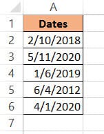
Suppose you have a data set as shown below, and you want to convert all these numbers in column A into the corresponding date that it represents.

Below are the steps to do this:
- Select the cells that have the number that you want to convert into a date

- Click the ‘Home’ tab

- In the ‘Number’ group, click on the Number Formatting drop-down

- In the drop-down, select ‘Long Date’ or Short Date’ option (based on what format would you want these numbers to be in)


That’s it!
The above steps would convert the numbers into the selected date format.

The above steps have not changed the value in the cell, only the way it’s being displayed.
Note that Excel picks up the short date formatting based on your system’s regional setting. For example, if you’re in the US, then the date format would be MM/DD/YYYY, and if you are in the UK, then the date format would be DD/MM/YYYY.
While this is a quick method to convert serial numbers into dates, it has a couple of limitations:
- There are only two date formats – short date and long date (and that too in a specific format). So, if you want to only get the month and the year and not the day, you won’t be able to do that using these options.
- You cannot show date as well as time using the formatting options in the drop-down. You can either choose to display the date or the time but not both.
So, if you need more flexibility in the way you want to show dates in Excel, you need to use the Custom Number Formatting option (covered next in this tutorial).
Sometimes when you convert a number into a date in Excel, instead of the date you may see some hash signs (something like #####). this happens when the column width is not enough to accommodate the entire date. In such a case, just increase the width of the column.
Creating a Custom Date Format Using Number Formatting Dialog Box
Suppose you have a data set as shown below and you want to convert the serial numbers in column A into dates in the following format – 01.01.2020
Note that this option is not available by default in the ribbon method that we covered earlier.
Below are the steps to do this:
- Select the cells that have the number that you want to convert into a date
- Click the ‘Home’ tab
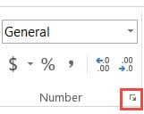
- In the Numbers group, click on the dialog box launcher icon (it’s a small tilted arrow at the bottom right of the group)

- In the ‘Format Cells’ dialog box that opens up, make sure the ‘Number’ tab selected

- In the ‘Category’ options on the left, select ‘Date’
- Select the desired formatting from the ‘Type’ box.
- Click OK


The above steps would convert the numbers into the selected date format.

As you can see, there are more date formatting options in this case (as compared with the short and long date we got with the ribbon).
And in case you do not find the format you are looking for, you can also create your own date format.
For example, let’s say that I want to show the date in the following format – 01/01/2020 (which is not already an option in the format cells dialog box).
Here is how I can do this:
- Select the cells that have the numbers that you want to convert into a date
- Click the Home tab
- In the Numbers group, click on the dialog box launcher icon (it’s a small tilt arrow at the bottom right of the group)
- In the ‘Format Cells’ dialog box that opens up, make sure the ‘Number’ tab selected
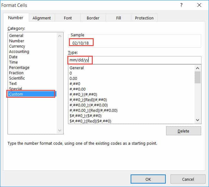
- In the ‘Category’ options on the left, select ‘Custom’
- In the field on the right, enter
mm/dd/yyyy
- Click OK


The above steps would change all the numbers into the specified number format.

With custom format, you get full control and it allows you to show the date in whatever format you want. You can also create a format where it shows the date as well time in the same cell.
For example, in the same example, if you want to show date as well as time, you can use the below format:
mm/dd/yyyy hh:mm AM/PM
Below is the table that shows the date format codes you can use:
| Date Formatting Code | How it Formats the Date |
| m | Shows the Month as a number from 1–12 |
| mm | Show the months as two-digit numbers from 01–12 |
| mmm | Shows the Month as three-letter as in Jan–Dec |
| mmmm | Shows the Months full name as in January–December |
| mmmmm | Shows the Month name first alphabet as in J-D |
| d | Shows Days as 1–31 |
| dd | Shows Days as 01–31 |
| ddd | Shows Days as Sun–Sat |
| dddd | Shows Days as Sunday–Saturday |
| yy | Shows Years as 00–99 |
| yyyy | Shows Years as 1900–9999 |
Also read: How to Convert Text to Date in Excel (Easy Formulas)
Convert Serial Numbers to Dates Using TEXT Formula
The methods covered above work by changing the formatting of the cells that have the numbers.
But in some cases, you may not be able to use these methods.
For example, below I have a data set where the numbers have a leading apostrophe – which converts these numbers into text.

If you try and using the inbuilt options to change the formatting of the cells with this data set, it would not do anything. This is because Excel does not consider these as numbers, and since dates for numbers, Excel refuses your wish to format these.
In such a case, you can either convert these text to numbers and then use the above-covered formatting methods, or use another technique to convert serial numbers into dates – using the TEXT function.
The TEXT function takes two arguments – the number that needs to be formatted, and the format code.
Suppose you have a data set as shown below, and you want to convert all the numbers and column A into dates.

Below the formula that could do that:
=TEXT(A2,"MM/DD/YYYY")
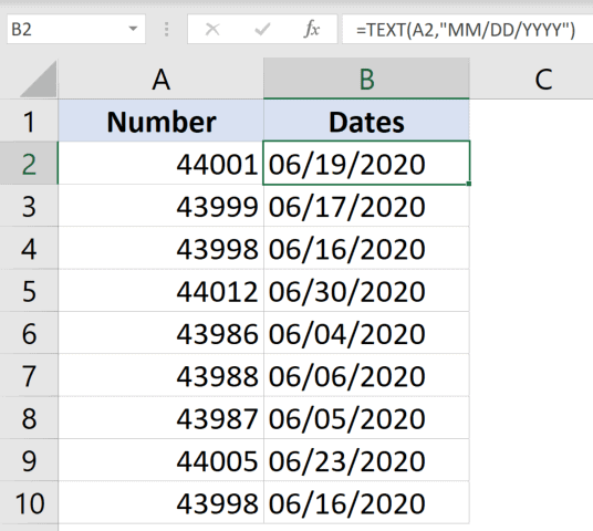
Note that in the formula I have specified the date formatting to be in the MM/DD/YYYY format. If you need to use any other formatting, you can specify the code for it as the second argument of the TEXT formula.
You can also use this formula to show the date as well as the time.
For example, if you want the final result to be in the format – 01/01/2020 12:00 AM, use the below formula:
=TEXT(A2,"mm/dd/yyyy hh:mm AM/PM")
In the above formula, I have added the time format as well so if there are decimal parts in the numbers, it would be shown as the time in hours and minutes.
If you only want the date (and not the underlying formula), convert the formulas into static values by using paste special.
One big advantage of using the TEXT function to convert serial numbers into dates is that you can combine the TEXT formula result with other formulas. For example, you can combine the resulting date with the text and show something such as – The Due Date is 01-Jan-2020 or The Deadline is 01-Jan-2020
Note: Remember dates and time are stored as numbers, where every integer number would represent one full day and the decimal part would represent that much part of the day. So 1 would mean 1 full day and 0.5 would mean half-a-day or 12 hours.
So these are two simple ways you can use to convert serial numbers to dates in Microsoft Excel.
I hope you found this tutorial useful!
Other Excel tutorials you may like:
- How to SUM values between two dates (using SUMIFS formula)
- How to Stop Excel from Changing Numbers to Dates Automatically
- How to Remove Time from Date/Timestamp in Excel
- Calculate the Number of Months Between Two Dates in Excel
- Excel DATEVALUE Function – Convert Date in Text into Serial Date Formats
- How to Convert Numbers to Text in Excel
- How to Compare Dates in Excel (Greater/Less Than, Mismatches)
- Convert Scientific Notation to Number or Text in Excel
- How To Convert Date To Serial Number In Excel?
How to Change Excel Date Format?
Excel date format related function are grouped in Menu-> Formula -> Date & Time Option.
Using this, we can get today’s date & time, calculate time differences, format date & time as per our needs. Lets start to learn some basics with Date and Time formula that are available within Excel under these titles.
- Get Excel VBA Today Date Functions.
- Excel Convert Number to Date
- Excel VBA Date Format conversion
- Excel Date Format Formula
1. Excel VBA Date Today
To get Excel today’s date use one of the following formula in any worksheet.
- “=Today()” : will fetch current date from System clock and display in the cell.
- “=Now()”: This command will fetch the date along with time from the system clock.
VBA Format Date Time
- VBA.Date : To get Excel VBA date today
- VBA.Now : To get VBA date & current tim
Sample Output from =Now() formula. ‘3/4/2014 15:02’. With “=Today()” command, only date will be displayed without time.
This function is explained here, as we need a sample Today’s date in Excel to test the methods explained under this article.
2. Excel Convert Number to Date or Date to String
Choose the cell that has data & use the Excel date format conversion as explained below.
- Select Excel cell that has Date.
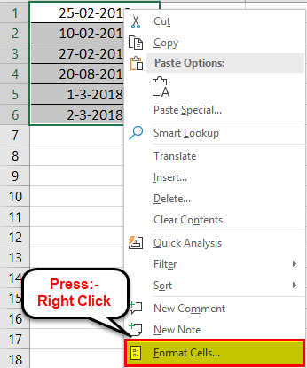
- Right Click & choose “Format Cells” (short cut – ‘CTRL + 1’).
- Choose ‘Number’ tab.
- Click ‘Custom’ under ‘Category’ list.
- Enter required format under ‘Type’ or choose a format in any of the defined types.
- Click ‘Ok’ to complete date formatting changes.
The selected cell will reflect the date format changes and display in the chosen format. This is not only for date, any number can be customized to a desired format using this option.
Remember that it does not change the way Excel stores the data. This formatting changes only the display format.
3. Excel VBA Date Format
Use VBA date format codes explained in the below sample code inside your Excel macro.
In these sample, there are 4 different methods explained and it only converts the display of Excel VBA date format, not the actual data. It can be considered as converting number to date or string to date, only the visible mode.
Sub Excel_VBA_Date_Format()
    'Display Date Format in Selection  - Jul/21/2016
    Selection.NumberFormat = "mmm/d/yyyy"

    'Display Date Format in Cell Reference  - Thursday, July 21, 2016
    ThisWorkbook.Sheets(1).Cells(1, 12).NumberFormat = "[$-409]dddd, mmmm dd, yyyy"

    'Display Date Format using WorksheetFunction  - Thursday, July 21, 2016
    ThisWorkbook.Sheets(2).Cells(2, 12) = Application.WorksheetFunction.Text(42572, "dddd mmmm-dd-yyyy")

    'Display Date Format using WorksheetFunction inside Cell - Thursday, July 21, 2016
    ThisWorkbook.Sheets(2).Cells(3, 12) = "=TEXT(42573,""mmmm/dd/yyyy"")"
End Sub
Enter different date formats in a new Excel workbook & try the above code to learn how each line make date format conversions.
4. Excel Date Format Formula
Consider the sample date & time value we got from above formulas to explore the available functions. To change this format from numeric date to text with month name like “04-Mar-14”. Then use this Excel Date format formula
- =TEXT(TODAY(),”dd-mmm-yyyy”) or
- =TEXT(NOW(),”dd-mmm-yyyy”)
To know other possible parameters or conversions that can be done using this formula, refer to the Wiki page mentioned at end of this article.
Excel Convert Number To Date – How Date is Stored in Excel?
It is enough to convert any date that is not in proper format to readable format with this “TEXT” function.
Before we convert any date, lets understand bit of basic behind how Excel stores the date in Worksheets. To do this, copy the output of Today(), Select another empty cell, right click, Paste Special, Choose Values and click ok. You could see some junk value or some random number.
What is it? It is the number of days from 1st January 1900 till date.
Excel will convert the dates entered into a number that equals number of days from 1-jan-1900. Excel uses this number in most of its Date calculations. To convert this back to a date, change the format of cells and choose date.
To know the date, month or year from this Date Serial number use the formula Date(), Month() or Year(). Similar to the Date, Time is also converted to a decimal.
Additional Reference
http://office.microsoft.com/en-in/excel-help/date-and-time-functions-reference-HP010342402.aspx
When you bring in data from other sources, it is not uncommon to get the dates in the form of serial numbers, like 42088.
Moreover, Excel inherently stores dates in the form of integers and then formats it according to the required date settings.
So when you apply certain formulas to dates or when you format a cell in the Number format, you often end up getting a serial number.
Although this form of storing dates seems unintuitive, it makes sense because it’s easier for Excel to perform various calculations with dates when in integer form.
Since it’s difficult for us humans to understand this date format though, it becomes necessary to convert these serial numbers to a recognizable date format.
In this tutorial, we will see three ways to convert a serial number to date format in Excel.
Understanding the Concept of Serial Numbers
Excel stores date in the form of integers or serial numbers. The serial starts from January 1, 1900, and increases by 1 for each day since then. That means January 1, 1900, has the serial 1, the next day has the serial 2, and so on.
In this way, the serial for June 1, 2019, is 43617, because it is exactly 43,617 days after January 1, 1900.
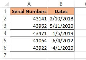
Throughout this tutorial, we are going to use the following set of date serial numbers.
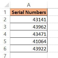
We will use the above three methods to convert these serial numbers to dates in different formats.
Method 1: Converting Serial Number to Date using the TEXT function
The TEXT function in Excel converts any numeric value (like date, time, and currency) into text with the given format. We can use this function to convert our serial number to any date format.
Here’s the syntax for the TEXT function:
= TEXT (serial_number, date_format_code)
In this function,
- serial_number is the numeric value or reference to the cell that you want to convert.
- date_format_code is the date format you want to convert the serial number to.
The TEXT function essentially applies the date_format_code that you specified on the provided serial_number and returns a text string with that format. For example, if you have the serial number “43141” in cell A2, then =TEXT(A2,”dd/mm/yy”) will return “10/02/18”
The format code will depend on the format that you want your converted date to appear. Here are some basic building blocks for the format codes that you can use:
Format Codes for Day of the Month:
You can use the following basic format codes to represent day values:
- d – one or two-digit representation of the day (eg: 3 or 30)
- dd – two-digit representation of the day (eg: 03 or 30)
- ddd – the day of the week in abbreviated form (eg: Sun, Mon)
- dddd – full name of the day of the week (eg: Sunday, Monday)
So,
- if you apply =TEXT(A2, “d”) to the sample dataset, it will return “10”.
- if you apply =TEXT(A2, “dd”), then it will return “10”.
- if you apply =TEXT(A2, “ddd”) to the sample dataset, it will return “Sat”.
- if you apply =TEXT(A2, “dddd”), then it will return “Saturday”.
Format Codes for Year:
You can use the following basic format codes to represent year values:
- yy – two-digit representation of year (e.g. 20 or 12)
- yyyy – four-digit representation of year (e.g. 2020 or 2012)
So,
- if you apply =TEXT(A2, “yy”) to the sample dataset, it will return “18”.
- if you apply =TEXT(A2, “yyyy”), then it will return “2018”.
Format Codes for Month of the Year:
You can use the following basic format codes to represent month values:
- m – one or two-digit representation of the month (eg; 8 or 12)
- mm – two-digit representation of the month (eg; 08 or 12)
- mmm – month abbreviated in three letters (eg: Aug or Dec)
- mmmm – month expressed with the full name (eg: August or December)
So,
- if you apply =TEXT(A2, “m”) to the sample dataset, it will return “2”.
- if you apply =TEXT(A2, “mm”), then it will return “02”.
- if you apply =TEXT(A2, “mmm”), then it will return “Feb”.
- if you apply =TEXT(A2, “mmmm”), then it will return “February”.
Let us see how we can apply the TEXT function to our sample dataset to convert all the serial numbers to different date formats.
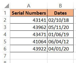
We will first see how to convert the serial numbers in column A to the format shown in column B in the image below:
Below are the steps to do this:
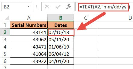
- Click on a blank cell where you want the converted date to be displayed (B2)
- Type the formula:
=TEXT(A2,”mm/dd/yy”).
- Press the Return key.
- This should display the serial number in our required date format. Copy this to the rest of the cells in the column by dragging down the fill handle or double-clicking on it.

- Copy this column’s formula results by pressing CTRL+C or Cmd+C (if you’re on a Mac).
- Right-click on the column and form the popup menu that appears, press Paste Values from the Paste Options.
- This will store the formula results as permanent values in the same column. Now you can go ahead and remove column A if you want to.

The result you get in column B will differ according to the format code you used in step 2. Here are some format codes along with the type of result you will get when applied to cell A2:
| Function | Result |
| =TEXT(A2, “dd/mm/yy”) | 02/10/18 |
| =TEXT(A2, “mm-dd-yy”) | 02-10-18 |
| TEXT(A2,”dddd, mmmm d, yyyy”)”) | Saturday, February 10, 2018 |
This means you can use the TEXT function to convert serial numbers to any date format of your choice. All you need to do is change the format_code according to your requirement.
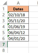
Note: Using this formula, your converted date is in text format. If you want to convert it to date format, you need to use the Format Cells feature.
Also read: How To Combine Date and Time in Excel (3 Easy Ways)
Method 2: Converting Serial Number to Date using Format Cells
This method makes use of Excel’s FormatCells dialog box. The Format Cells dialog box is very versatile and lets you perform different kinds of formatting from one place.
You can use Format Cells to convert the serial numbers in our sample dataset into dates as follows:
- Select all the cells containing the serial numbers that you want to convert (A2:A6).
- Right-click on your selection and select Format Cells from the popup menu that appears. Alternatively, you can select the dialog box launcher in the Number group under the Home tab.

- This will open the Format Cells dialog box. Click on the Number tab
- Under Category on the left side of the box, select the Date option.
- This will display a number of formatting options for the date on the right side.
- Select the format that you want.
- If you don’t find an option for the format you want to use, then you can use the Custom option from the Category list on the left. This lets you convert the cell to a custom date format.
- Check if your required date format is available among the format codes under Type. If not, you can type in your format code in the input box just below Type.
- Click OK to close the Format Cells dialog box.

All your selected cells should now be converted to date with your required format.
Note that these cells do not have the little green triangles at the top left corners. This is because these cells are of type date, and not text. So, you can perform any kind of date operations on them.
Also read: How to Add Minutes to Time in Excel?
Method 3: Converting Serial Number to date using VBA
If you’re comfortable with coding or using VBA, then you can use this method to quickly get all your serial numbers converted to date in one go.
Here’s the VBA code. You can copy and save this code somewhere for future use:
Sub convert_serial_num_to_date()
Dim rng As Range
Dim cell As Range
Set rng = Application.Selection
For Each cell In rng
cell.Offset(0, 1).Value = CDate(cell.Value)
Next cell
End Sub
Here are the steps you need to follow if you want to apply the above code to your dataset:
- From the Developer Menu Ribbon, select Visual Basic.
- Once your VBA window opens, Click Insert->Module. Now you can start coding. Type or copy-paste the above lines of code into the module window. Your code is now ready to run.
- Go to your worksheet and select the range of cells containing the serial numbers you want to convert. Make sure the column next to it is blank because this is where the code will display the results.
- Navigate to Developer->Macros-> convert_serial_num_to_date->Run.
You will now see the serial numbers converted to dates in the column next to your selection.
If you want to, you can now delete the original column containing the serial numbers.
In this tutorial, we saw three simple ways in which you can convert date serial numbers to actual dates in Excel. These included the use of the TEXT function, the Format Cells feature, and the VBA script.
Using the TEXT function usually results in cells that are of the text format so it requires subsequent conversion of these cells to the date format.
Using Format Cells, however, you can apply the operation directly on the original cells and the results you get are of the date type. So, you can directly start applying the cells to date-related operations. T
The VBA script that we provided in this tutorial used CDate() to quickly convert the serial number to its date equivalent. Moreover, the script results in cells that are of type date.
So again, it’s easier to use these results in subsequent date operations.
We hope you found the pointers we provided in this tutorial helpful and easy to apply.
Other Excel tutorials you may like:
- How to Convert Date to Month and Year in Excel
- How to Convert Decimal to Fraction in Excel
- How to Convert Radians to Degrees in Excel
- How to Add Days to a Date in Excel
- How to Sort by Date in Excel (Single Column & Multiple Columns)
- How to Convert Date to Day of Week in Excel
- How to Convert Month Number to Month Name in Excel
- Find Last Monday of the Month Date in Excel
- How to Change Date and Time to Date in Excel
It sometimes happens that we type or copy/paste date formats from sheets in Excel, but it displays as number. Let’s convert those 5-digits general numbers to date format with 2 easy steps using default date formatting function.
For example, we copied date from external source or wrote date in the cell but it displays in 5 digit number format as shown in the below screenshot:
Follow 2 easy steps to change 5 digit number format to date format.
Select the 5 digits numbers and click Number format box in Home Tab. Now select Short Date as shown below:
All selected 5 digits numbers converted to dates with default date formatting as shown below:
If you have any queries or suggestions, feel free to comment below. I will be happy to reply you.

I have worked in Excel and like to share functional excel templates at ExcelDataPro.
Introduction
Number formats control how numbers are displayed in Excel. The key benefit of number formats is that they change how a number looks without changing any data. They are a great way to save time in Excel because they perform a huge amount of formatting automatically. As a bonus, they make worksheets look more consistent and professional.
Video: What is a number format
What can you do with custom number formats?
Custom number formats can control the display of numbers, dates, times, fractions, percentages, and other numeric values. Using custom formats, you can do things like format dates to show month names only, format large numbers in millions or thousands, and display negative numbers in red.

Where can you use custom number formats?
Many areas in Excel support number formats. You can use them in tables, charts, pivot tables, formulas, and directly on the worksheet.
- Worksheet — format cells dialog
- Pivot Tables — via value field settings
- Charts — data labels and axis options
- Formulas — via the TEXT function
What is a number format?
A number format is a special code to control how a value is displayed in Excel. For example, the table below shows 7 different number formats applied to the same date, January 1, 2019:
| Input | Code | Result |
|---|---|---|
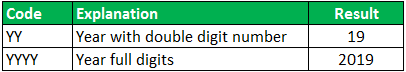
| 1-Jan-2019 | yyyy | 2019 |
| 1-Jan-2019 | yy | 19 |
| 1-Jan-2019 | mmm | Jan |
| 1-Jan-2019 | mmmm | January |
| 1-Jan-2019 | d | 1 |
| 1-Jan-2019 | ddd | Tue |
| 1-Jan-2019 | dddd | Tuesday |
The key thing to understand is that number formats change the way numeric values are displayed, but they do not change the actual values.
Where can you find number formats?
On the home tab of the ribbon, you’ll find a menu of build-in number formats. Below this menu to the right, there is a small button to access all number formats, including custom formats:

This button opens the Format Cells dialog box. You’ll find a complete list of number formats, organized by category, on the Number tab:

Note: you can open Format Cells dialog box with the keyboard shortcut Control + 1.
General is default
By default, cells start with the General format applied. The display of numbers using the General number format is somewhat «fluid». Excel will display as many decimal places as space allows, and will round decimals and use scientific number format when space is limited. The screen below shows the same values in column B and D, but D is narrower and Excel makes adjustments on the fly.

How to change number formats
You can select standard number formats (General, Number, Currency, Accounting, Short Date, Long Date, Time, Percentage, Fraction, Scientific, Text) on the home tab of the ribbon using the Number Format menu.
Note: As you enter data, Excel will sometimes change number formats automatically. For example if you enter a valid date, Excel will change to «Date» format. If you enter a percentage like 5%, Excel will change to Percentage, and so on.
Shortcuts for number formats
Excel provides a number of keyboard shortcuts for some common formats:
| Format | Shortcut |
|---|---|
| General format | Ctrl Shift ~ |
| Currency format | Ctrl Shift $ |
| Percentage format | Ctrl Shift % |
| Scientific format | Ctrl Shift ^ |
| Date format | Ctrl Shift # |
| Time format | Ctrl Shift @ |
| Custom formats | Control + 1 |
See also: 222 Excel Shortcuts for Windows and Mac
Where to enter custom formats
At the bottom of the predefined formats, you’ll see a category called custom. The Custom category shows a list of codes you can use for custom number formats, along with an input area to enter codes manually in various combinations.

When you select a code from the list, you’ll see it appear in the Type input box. Here you can modify existing custom code, or to enter your own codes from scratch. Excel will show a small preview of the code applied to the first selected value above the input area.
Note: Custom number formats live in a workbook, not in Excel generally. If you copy a value formatted with a custom format from one workbook to another, the custom number format will be transferred into the workbook along with the value.
How to create a custom number format
To create custom number format follow this simple 4-step process:
- Select cell(s) with values you want to format
- Control + 1 > Numbers > Custom
- Enter codes and watch preview area to see result
- Press OK to save and apply
Tip: if you want base your custom format on an existing format, first apply the base format, then click the «Custom» category and edit codes as you like.
How to edit a custom number format
You can’t really edit a custom number format per se. When you change an existing custom number format, a new format is created and will appear in the list in the Custom category. You can use the Delete button to delete custom formats you no longer need.
Warning: there is no «undo» after deleting a custom number format!
Structure and Reference
Excel custom number formats have a specific structure. Each number format can have up to four sections, separated with semi-colons as follows:

This structure can make custom number formats look overwhelmingly complex. To read a custom number format, learn to spot the semi-colons and mentally parse the code into these sections:
- Positive values
- Negative values
- Zero values
- Text values
Not all sections required
Although a number format can include up to four sections, only one section is required. By default, the first section applies to positive numbers, the second section applies to negative numbers, the third section applies to zero values, and the fourth section applies to text.
- When only one format is provided, Excel will use that format for all values.
- If you provide a number format with just two sections, the first section is used for positive numbers and zeros, and the second section is used for negative numbers.
- To skip a section, include a semi-colon in the proper location, but don’t specify a format code.
Characters that display natively
Some characters appear normally in a number format, while others require special handling. The following characters can be used without any special handling:
| Character | Comment |
|---|---|
| $ | Dollar |
| +- | Plus, minus |
| () | Parentheses |
| {} | Curly braces |
| <> | Less than, greater than |
| = | Equal |
| : | Colon |
| ^ | Caret |
| ‘ | Apostrophe |
| / | Forward slash |
| ! | Exclamation point |
| & | Ampersand |
| ~ | Tilde |
| Space character |
Escaping characters
Some characters won’t work correctly in a custom number format without being escaped. For example, the asterisk (*), hash (#), and percent (%) characters can’t be used directly in a custom number format – they won’t appear in the result. The escape character in custom number formats is the backslash (). By placing the backslash before the character, you can use them in custom number formats:
| Value | Code | Result |
|---|---|---|
| 100 | #0 | #100 |
| 100 | *0 | *100 |
| 100 | %0 | %100 |
Placeholders
Certain characters have special meaning in custom number format codes. The following characters are key building blocks:
| Character | Purpose |
|---|---|
| 0 | Display insignificant zeros |
| # | Display significant digits |
| ? | Display aligned decimals |
| . | Decimal point |
| , | Thousands separator |
| * | Repeat following character |
| _ | Add space |
| @ | Placeholder for text |
Zero (0) is used to force the display of insignificant zeros when a number has fewer digits than zeros in the format. For example, the custom format 0.00 will display zero as 0.00, 1.1 as 1.10 and .5 as 0.50.

Pound sign (#) is a placeholder for optional digits. When a number has fewer digits than # symbols in the format, nothing will be displayed. For example, the custom format #.## will display 1.15 as 1.15 and 1.1 as 1.1.

Question mark (?) is used to align digits. When a question mark occupies a place not needed in a number, a space will be added to maintain visual alignment.

Period (.) is a placeholder for the decimal point in a number. When a period is used in a custom number format, it will always be displayed, regardless of whether the number contains decimal values.
Comma (,) is a placeholder for the thousands separators in the number being displayed. It can be used to define the behavior of digits in relation to the thousands or millions digits.

Asterisk (*) is used to repeat characters. The character immediately following an asterisk will be repeated to fill remaining space in a cell.

Underscore (_) is used to add space in a number format. The character immediately following an underscore character controls how much space to add. A common use of the underscore character is to add space to align positive and negative values when a number format is adding parentheses to negative numbers only. For example, the number format «0_);(0)» is adding a bit of space to the right of positive numbers so that they stay aligned with negative numbers, which are enclosed in parentheses.

At (@) — placeholder for text. For example, the following number format will display text values in blue:
0;0;0;[Blue]@
See below for more information about using color.
Automatic rounding
It’s important to understand that Excel will perform «visual rounding» with all custom number formats. When a number has more digits than placeholders on the right side of the decimal point, the number is rounded to the number of placeholders. When a number has more digits than placeholders on the left side of the decimal point, extra digits are displayed. This is a visual effect only; actual values are not modified.
Number formats for TEXT
To display both text along with numbers, enclose the text in double quotes («»). You can use this approach to append or prepend text strings in a custom number format, as shown in the table below.
| Value | Code | Result |
|---|---|---|
| 10 | General» units» | 10 units |
| 10 | 0.0″ units» | 10.0 units |
| 5.5 | 0.0″ feet» | 5.5 feet |
| 30000 | 0″ feet» | 30000 feet |
| 95.2 | «Score: «0.0 | Score: 95.2 |
| 1-Jun | «Date: «mmmm d | Date: June 1 |
Number formats for DATES
Dates in Excel are just numbers, so you can use custom number formats to change the way they display. Excel has many specific codes you can use to display components of a date in different ways. The screen below shows how Excel displays the date in D5, September 3, 2018, with a variety of custom number formats:

Number formats for TIME
Times in Excel are fractional parts of a day. For example, 12:00 PM is 0.5, and 6:00 PM is 0.75. You can use the following codes in custom time formats to display components of a time in different ways. The screen below shows how Excel displays the time in D5, 9:35:07 AM, with a variety of custom number formats:

Note: m and mm can’t be used alone in a custom number format since they conflict with the month number code in date format codes.
Number formats for ELAPSED TIME
Elapsed time is a special case and needs special handling. By using square brackets, Excel provides a special way to display elapsed hours, minutes, and seconds. The following screen shows how Excel displays elapsed time based on the value in D5, which represents 1.25 days:

Number formats for COLORS
Excel provides basic support for colors in custom number formats. The following 8 colors can be specified by name in a number format: [black] [white] [red][green] [blue] [yellow] [magenta] [cyan]. Color names must appear in brackets.

Colors by index
In addition to color names, it’s also possible to specify colors by an index number (Color1,Color2,Color3, etc.) The examples below are using the custom number format: [ColorX]0″▲▼», where X is a number between 1-56:
[Color1]0"▲▼" // black
[Color2]0"▲▼" // white
[Color3]0"▲▼" // red
[Color4]0"▲▼" // green
etc.
The triangle symbols have been added only to make the colors easier to see. The first image shows all 56 colors on a standard white background. The second image shows the same colors on a gray background. Note the first 8 colors shown correspond to the named color list above.


Apply number formats in a formula
Although most number formats are applied directly to cells in a worksheet, you can also apply number formats inside a formula with the TEXT function. For example, with a valid date in A1, the following formula will display the month name only:
=TEXT(A1,"mmmm")
The result of the TEXT function is always text, so you are free to concatenate the result of TEXT to other strings:
="The contract expires in "&TEXT(A1,"mmmm")
The screen below shows the number formats in column C being applied to numbers in column B using the TEXT function:

One quirk of the TEXT function relates to double quotes («») that are part of certain custom number formats. Because the format_text is entered as a text string, Excel won’t allow you to enter the formula without removing the quotes or adding more quotes. For example, to display a large number in thousands, you can use a custom number format like this:
0, "k"Notice k appears in quotes («k»). To apply the same format with the TEXT function, you can use simply:
=TEXT(A1,"0, k")Notice the k is not surrounded by quotes. Alternately, you can add extra double quotes as below, which returns the same result:
=TEXT(A1,"0,""K""")This behavior only occurs when you are hardcoding a format inside TEXT. If you are applying a format entered elsewhere on the worksheet (as in cells C6 and C9 in the worksheet above) you can use a standard number format.
Measurements
You can use a custom number format to display numbers with an inches mark («) or a feet mark (‘). In the screen below, the number formats used for inches and feet are:
0.00 ' // feet
0.00 " // inches

These results are simplistic, and can’t be combined in a single number format. You can however use a formula to display feet together with inches.
Conditionals
Custom number formats also up to two conditions, which are written in square brackets like [>100] or [<=100]. When you use conditionals in custom number formats, you override the standard [positive];[negative];[zero];[text] structure. For example, to display values below 100 in red, you can use:
[Red][<100]0;0
To display values greater than or equal to 100 in blue, you can extend the format like this:
[Red][<100]0;[Blue][>=100]0

To apply more than two conditions, or to change other cell attributes, like fill color, etc. you’ll need to switch to Conditional Formatting, which can apply formatting with much more power and flexibility using formulas.
Plural text labels
You can use conditionals to add an «s» to labels greater than zero with a custom format like this:
[=1]0″ day»;0″ days»

Telephone numbers
Custom number formats can also be used for telephone numbers, as shown in the screen below:

Notice the third and fourth examples use a conditional format to check for numbers that contain an area code. If you have data that contains phone numbers with hard-coded punctuation (parentheses, hyphens, etc.) you will need to clean the telephone numbers first so that they only contain numbers.
Hide all content
You can actually use a custom number format to hide all content in a cell. The code is simply three semi-colons and nothing else ;;;
To reveal the content again, you can use the keyboard shortcut Control + Shift + ~, which applies the General format.
Other resources
- Developer Bryan Braun built a nice interactive tool for building custom number formats
What is the Date Format in Excel?
In Excel, a date is displayed according to the format selected by the user. One can choose from the different formats available or create a customized format according to the requirement. The default date format is specified in the “Control Panel” of the system. However, it is possible to change these default settings.
For example, the date 01/01/2021 corresponds to the format dd/mm/yyyy. If the format is changed to d-mmm-yyyy, the date becomes 1-Jan-2021.
We can change the date format in Excel either from the “Number Format” of the “Home” tab or the “Format Cells” option of the context menu.
In Excel for Windows, 1900 is the default date system. Whereas, in Excel for Mac, 1904 is the default date system. Both these systems store the dates as consecutive numbers having a difference of 1. These numbers are known as serial values or serial numbers. The reason dates are stored as serial numbers is to facilitate calculations.
In the 1900 date system, the first date that Excel recognizes is January 1, 1900. This date is stored as the number 1 in Excel. Consequently, the number 2 represents January 2, 1900. The last date recognized by Excel is December 31, 9999. It is represented by the serial number 2958465. Date before 1900 or after 9999 is identified as a text value by Excel.
Dates are stored only as positive integers in the 1900 date system. However, to display negative numbers as negative dates, one needs to switch to the 1904 date system.
In the 1904 date system, 0 represents January 1, 1904, and -1 means January -2, 1904. The number 1 represents January 2, 1904. The last date recognized by Excel (in the 1904 date system) is December 31, 9999, represented by the serial number 2957003.
In this article, we follow the 1900 date system.
Table of contents
- What is theDate Format in Excel?
- Code of Date Format in Excel
- How to Change Date Format in Excel?
- Example #1–Apply Default Format of Long Date in Excel
- Example #2–Change the Date Excel Format Using “Custom” Option
- Example #3–Apply Different Types of Customized Date Formats in Excel
- Example #4–Convert Text Values Representing Dates to Actual Dates
- Example #5–Change the Date Format Using “Find and Replace” Box
- Frequently Asked Questions
- Recommended Articles
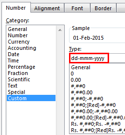
Code of Date Format in Excel
A code (like dd-mm-yyyy) is a representation of a day (d), month (m), and year (y). We can change the appearance of the date by changing the specified code.
The different codes, their explanation, and output (for days, months, and years) have been presented in the following images.
Notations for a Day

Notations for a Month

Notations for a Year
How to Change Date Format in Excel?
Here we look at some of the date format examples in Excel and how to change them.
Example #1–Apply Default Format of Long Date in Excel
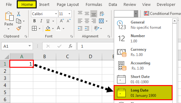
The following image shows a number in cell A1. We want to know the date represented by this number. The output should be in the long date format of Excel.
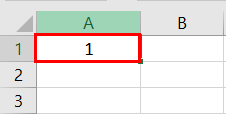
The steps to know the date represented by the number in cell A1 are listed as follows:
- We must first select cell A1. Then, from the “Home” tab, click the “Number Format” drop-down appearing in the “Number” section. Next, select “Long Date,” shown in the following image.

- The output is shown in the following image. The long date format displayed is dd mmmm yyyy. Hence, the number 1 represents the date 01 January 1900 in the long date format.
Note: The short and long dates appear as set in the “Control Panel.” Click “Clock, Language, and Region” in the “Control Panel” to change these default date formats. After that, click “Change date, time, or number formats.” Make the desired changes and click “OK.”
Likewise, had there been 2 in cell A1, the long date format would have been 02 January 1900. The number 3 would have been displayed as 03 January 1900 in the long date format.
Note: To switch to the 1904 date system, we must select “Advanced” from the “Options” of the “File” tab. Under “When calculating this workbook,” select “use 1904 date system” and click “OK.”

You can download this Change Date Format Excel Template here – Change Date Format Excel Template
Example #2–Change the Date Excel Format Using “Custom” Option
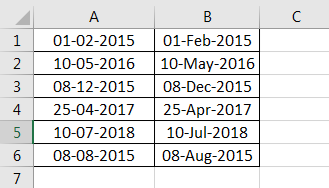
The following image shows some dates in the range A1:A6. These dates are in the format dd-mm-yyyy. We want to change their format to dd-mmmm-yyyy.
For instance, the date in cell A1 should appear as 25-February-2018. We may use the “Custom” option of the “Format Cells” dialog box.

The steps to change the date format in Excel are listed as follows:
Step 1: We need to select all the dates of the range A1:A6. The same is shown in the following image.
Step 2: We must right-click the selection and choose “Format Cells” from the context menu. Alternatively, we may also press the keys “Ctrl+1” together.
Step 3: The “Format Cells” window opens, as shown in the following image.
Note: The default short date and long date formats are marked with an asterisk (*) in the box under “type.” The short date is 3/14/2012 (m/dd/yyyy), and the long date is Wednesday, March 14, 2012 (dddd, mmmm dd, yyyy).
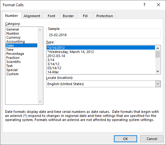
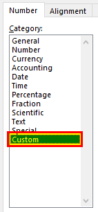
Step 4: From the “Number” tab, we need to select “Custom” under “Category.” The categories are shown on the left side of the “Format Cells” window.
Step 5: Under “Type,” we must insert the required date format. Either type the format (dd-mmmm-yyyy) or select it from the various options displayed in the box below “Type.”
Once the format has been entered, check the preview of the first date (of the range A1:A6) under “Sample.” The same is shown in the following image. Click “OK” in the “Format Cells” window if the date preview looks good.
Note 1: The date under “Sample” is displayed according to the format specified under “Type.”
Note 2: While creating custom date formats, we can use a forward slash (/), hyphen (-), comma (,), space ( ), etc.

Step 6: The output is shown in the following image. All dates of the range A1:A6 have been converted to the format dd-mmmm-yyyy. However, the Excel formula bar can still see the default date format. This default format corresponds with the short date set in the “Control Panel.”

Example #3–Apply Different Types of Customized Date Formats in Excel
The next image shows certain dates in the range A1:A6. At present, the date format is dd-mm-yyyy.
We want to apply four different formats to these dates. For using each format, the common steps to be performed are given as follows:
- First, we must select the range A1:A6.
- Then, right-click the selection and choose “Format Cells.”
- After that, from the “Number” tab, select “Custom” under “Category.”
Further, under each format, the additional steps to be performed followed by two images are given.

Format 1: dd-mmm-yyyy
- In the “Custom” option of the “Number” tab, select the format “dd-mmm-yyyy” under “Type.”
- Click “Ok.”

The output is given in the following image. All dates are displayed according to the format dd-mmm-yyyy. The hyphen is the separator between the day, month, and year in this format.

Format 2: dd mmm yyyy
- We must select the format “dd mmm yyyy” under “Type” of the “custom” option.
- Click “Ok.”

The output is given in the following image. All dates are converted to the format dd mmm yyyy. The space is the only separator between the day, month, and year in this format.

Format 3: ddd mmm yyyy
- In the “Custom” option, select the format “ddd mmm yyyy” under “Type.”
- Click “Ok.”

The output is given in the following image. The dates are shown in the format ddd mmm yyyy. The day and the month are displayed in their short notations in this format.

Format 4: dddd mmmm yyyy
- From the “Custom” option of the “Number” tab, select “dddd mmmm yyyy” under “Type.”
- Click “Ok.”

The output is given in the following image. All dates have been converted to the format dddd mmmm yyyy. The date, month, and year are displayed in their respective full forms in this format.

It must be observed that the date format changes as per the style set by the user. Therefore, the user can select a date format according to their convenience.
Example #4–Convert Text Values Representing Dates to Actual Dates
The following image shows a list of dates in the range A1:A6. At present, these dates are appearing as text values. We want to convert these text values to dates having the format dd-mmm-yyyy.

The steps to convert text values to dates having the given format are listed as follows:
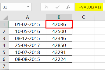
Step 1: First, enter the following formula in cell B1.
“=VALUE(A1)”
Then, press the “Enter” key.
Note 1: The VALUE functionIn Excel, the value function returns the value of a text representing a number. So, if we have a text with the value $5, we can use the value formula to get 5 as a result, so this function gives us the numerical value represented by a text.read more returns the numeric form of a text string that represents a number. In other words, it converts a number looking like the text into an actual number.
Note 2: Instead of the VALUE function, one can also use the DATEVALUE functionThe DATEVALUE function in Excel shows any given date in absolute format. This function takes an argument in the form of date text normally not represented by Excel as a date and converts it into a format that Excel can recognize as a date.read more of Excel. The latter converts a date stored as text to a serial number. This serial number is recognized as a date by Excel.
Step 2: We must select cell B1 and drag the fill handle until cell B6. The output is shown in the following image. All text values (A1:A6) have been converted to numbers (in the range B1:B6).
Ideally, the text string in Excel is left-aligned while the number string is right-aligned. However, we have centrally aligned both the ranges (A1:A6 and B1:B6).
Note: When text strings representing dates have been converted to serial values (or dates), we can use them for performing different calculations like addition, subtraction, and so on.
Step 3: To view the obtained serial numbers (in column B) as dates, apply the required format. We must select the range B1:B6, right-click and choose “Format Cells.”
In the “Number” tab, select the option “Custom.” Then, under “Type,” enter or choose the format “dd-mmm-yyyy.” The same is shown in the following image.
If the sample date looks alright, click “OK.”
Step 4: The output is shown in the following image. Hence, all text values (of column A) have been converted to valid dates (in column B) having the format dd-mmm-yyyy.
Note: To ensure that a value is recognized as a date by Excel, check for the following signs:
- The dates are right-aligned as they are numerical values.
- If two or more dates are selected, the status bar (at the bottom of the worksheet) shows the count, average, numerical count, and sum. In addition, it may display one or more options according to the Excel version.
If a value is a text string, it would be left-aligned, and the status bar will show only the count.
Often, the Excel date format needs to be changed (from text to dates) when data is downloaded (or copied and pasted) from the web. That is because, in such instances, the dates may not be displayed as numbers.
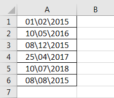
Example #5–Change the Date Format Using “Find and Replace” Box
The following image shows some text values representing dates in the range A1:A6. The days, months, and numbers have been separated with a backslash. That is because we want to perform the following tasks:
- Replace all the backslashes () with forwarding slashes (/) by using the “Find and Replace” dialog box.
- Convert text values representing dates to actual dates.
The steps to perform the given tasks are listed as follows:
Step 1: We must press the keys “Ctrl+H” together. Then, the “find and replace” dialog box opens, as shown in the following image.
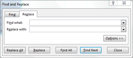
Step 2: Type a backslash in the “Find what” box (). In the “Replace with” box, type a forward slash (/).
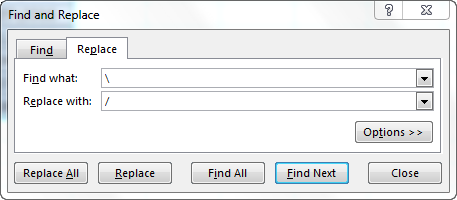
Step 3: Next, we must click “Replace All.” Excel shows a message stating the number of replacements it has made. Click “OK” to proceed. The final output is shown in the following image.
Hence, all backslashes have been replaced with forwarding slashes. With this replacement, the text values representing dates have automatically been converted to actual dates by Excel.
Since column A was aligned centrally from the beginning, this alignment is retained even after the values are converted to dates.

Frequently Asked Questions
1. How can the date format in Excel be changed?
The steps to change the date format in Excel are listed as follows:
The steps to change the date format in Excel are listed as follows:
a. Select the cell containing the date. If the date format of a range needs to be changed, select the entire range.
b. Right-click the selection and choose “Format Cells” from the context menu. Alternatively, press the keys “Ctrl+1” together.
c. IIn the “Number” tab, select the option “Date.” Next, select the required date format under “Type.”
d. Check the preview (of the first date of the selected range) under “Sample.” If the preview is good, click “OK.”
The date format of the selected cell or cells (selected in step a) is changed.
Note 1: The required date format may not be available under the “Date” option’s “Type.” If it is not available, select “Custom” as the “category” from the “Number” tab. Then, type the required date format under “Type” and click “OK.”
Note 2: If the selected cell (selected in step a) contains a text string representing a date, convert this string to date first. Then change the format to the desired date format.
2. How to change the date format permanently in Excel?
To change a date format permanently, one needs to make changes to the date formats of the “Control Panel.” That is because the short and long date formats of Excel reflect the date settings of the “Control Panel.”
The steps to change the date settings of the “Control Panel” are listed as follows:
We must open the “Control Panel” first from the “Start” menu.
b. In the “Clock, Language, and Region” category, click “Change date, time, or number format.” It is available under the “Region and Language” option.
c. The “Region and Language” or “Region” dialog box opens. Under “Format,” we must select the region.
d. Enter the required short and long date formats under “Date and Time Formats.” To enter customized short and long date formats, click “Additional Settings.” The “Customize Format” dialog box opens. Make the changes in the “Date” tab and click “OK.”
e. Check the preview under “Examples” at the bottom of the “Region and Language” box. If the preview is alright, click “OK.”
The default date settings have been changed. Now, we should enter a date in any format in Excel. Then select the short or the long date format from the “Number Format” (in the “Number” section) of the “Home” tab.
The dates will appear in the format set in the “Control Panel.” So, the user need not change the format of each date manually.
3. How to change a date to a text string in Excel?
Let us change the date 22/1/2019 in cell A1 to a text string in Excel. The text string should be in the format yyyy-mm-dd.
The steps to change a date to a text string are listed as follows:
a. First, we must enter the formula =TEXT(A1, “yyyy-mm-dd”) in cell B1.
b. Then, press the “Enter” key.
The date in cell A1 (22/1/2019) is converted to 2019-01-22 in cell B1. We must note that the date in cell A1 is right-aligned, being a number. In contrast, the text in cell B1 is left-aligned.
Note: The TEXT function helps convert numbers to text strings. It is used to display values in a specific format. The syntax is TEXT(value,format_text). “Value” is the number to be converted to text. “Format_text” is the format in which the number should be displayed.
Recommended Articles
This article has been a guide to the Date Format in Excel. We discuss changing and customizing date formats in Excel, practical examples, and a downloadable Excel template. You may also look at these useful functions in Excel: –
- Concatenate Columns in Excel
- Convert Date to Text in Excel
- Insert Date in Excel
- Concatenate Date in Excel