
IF function
The IF function is one of the most popular functions in Excel, and it allows you to make logical comparisons between a value and what you expect.
So an IF statement can have two results. The first result is if your comparison is True, the second if your comparison is False.
For example, =IF(C2=”Yes”,1,2) says IF(C2 = Yes, then return a 1, otherwise return a 2).

Use the IF function, one of the logical functions, to return one value if a condition is true and another value if it’s false.
IF(logical_test, value_if_true, [value_if_false])
For example:
-
=IF(A2>B2,»Over Budget»,»OK»)
-
=IF(A2=B2,B4-A4,»»)
|
Argument name |
Description |
|---|---|
|
logical_test (required) |
The condition you want to test. |
|
value_if_true (required) |
The value that you want returned if the result of logical_test is TRUE. |
|
value_if_false (optional) |
The value that you want returned if the result of logical_test is FALSE. |
Simple IF examples

-
=IF(C2=”Yes”,1,2)
In the above example, cell D2 says: IF(C2 = Yes, then return a 1, otherwise return a 2)

-
=IF(C2=1,”Yes”,”No”)
In this example, the formula in cell D2 says: IF(C2 = 1, then return Yes, otherwise return No)As you see, the IF function can be used to evaluate both text and values. It can also be used to evaluate errors. You are not limited to only checking if one thing is equal to another and returning a single result, you can also use mathematical operators and perform additional calculations depending on your criteria. You can also nest multiple IF functions together in order to perform multiple comparisons.

-
=IF(C2>B2,”Over Budget”,”Within Budget”)
In the above example, the IF function in D2 is saying IF(C2 Is Greater Than B2, then return “Over Budget”, otherwise return “Within Budget”)

-
=IF(C2>B2,C2-B2,0)
In the above illustration, instead of returning a text result, we are going to return a mathematical calculation. So the formula in E2 is saying IF(Actual is Greater than Budgeted, then Subtract the Budgeted amount from the Actual amount, otherwise return nothing).

-
=IF(E7=”Yes”,F5*0.0825,0)
In this example, the formula in F7 is saying IF(E7 = “Yes”, then calculate the Total Amount in F5 * 8.25%, otherwise no Sales Tax is due so return 0)
Note: If you are going to use text in formulas, you need to wrap the text in quotes (e.g. “Text”). The only exception to that is using TRUE or FALSE, which Excel automatically understands.
Common problems
|
Problem |
What went wrong |
|---|---|
|
0 (zero) in cell |
There was no argument for either value_if_true or value_if_False arguments. To see the right value returned, add argument text to the two arguments, or add TRUE or FALSE to the argument. |
|
#NAME? in cell |
This usually means that the formula is misspelled. |
Need more help?
You can always ask an expert in the Excel Tech Community or get support in the Answers community.

See Also
IF function — nested formulas and avoiding pitfalls
IFS function
Using IF with AND, OR and NOT functions
COUNTIF function
How to avoid broken formulas
Overview of formulas in Excel
Need more help?
Maintenance Alert: Saturday, April 15th, 7:00pm-9:00pm CT. During this time, the shopping cart and information requests will be unavailable.
Categories: Conditional Formatting, Excel®
Tags: If/Then Conditional formatting
*Steps in this article will apply to Excel 2007-2016. Images were taken using Excel 2016.
If you are a fan of Excel’s conditional formatting feature, you probably find looking for even more and more ways to highlight useful information in your data. A question that often comes up among these “conditional formatting addicts” is Can I use If/Then formula to format a cell?
The answer is yes and no. Any conditional formatting argument must generate a TRUE result, meaning that at a literal level, your conditional formatting rule is an If/Then statement along the lines of “If this condition is TRUE, THEN format the cell this way”.
What conditional formatting can’t do in a single rule is an IF/THEN/ELSE condition such as “If # is greater than 10 format red, else format green”. Instead, this would require TWO rules, one for “greater than 10” and one for “less than 10”.
Let’s look at a few scenarios to get a sense of how we can create the effect of IF/THEN conditional formatting, even if we can’t use it in the feature itself:
To follow using our examples, download 04-If-Then Conditional Formatting.xlsx
Scenario 1 (Birthdays tab): You want to highlight all employees in your department who have a birthday this month with Red, and all other departments blue.
Solution: Create two rules – one for your department, one for all others
Step 1 – Highlight birthdays in your department
The formula to identify birthdays in the current month will be (see this article for more about using dates in conditional formatting):
=MONTH(C2)=MONTH(TODAY())
To create a formula that generates a TRUE/FALSE statement that highlights birthdays only in one department, you would use the formula:
=AND(MONTH(C2)=MONTH(TODAY()),D2=”Sales”)
This example was created in April, so April birthdays will be highlighted. If you are reproducing the exercise in a different month, you will see different results!
Then, create a second rule for the same range using this formula to highlight birthdays that are not in your department:
=AND(MONTH(C1)=MONTH(TODAY()),D1<>”Sales”)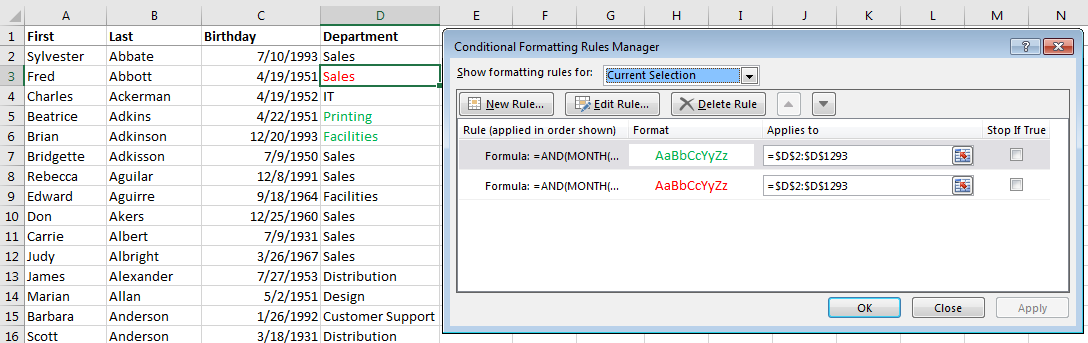
BONUS! In this example, we applied the rule to the department cell to show the relationship to the formula. By changing the Applies to range, however, you can easily highlight a different cell – such as the birthdate – or the entire row. See Get the Most Out of Excel’s Conditional Formatting for more ideas.
Scenario 2 (Retainers tab): You have a table of how many hours your employees have worked for specific clients, and you have a table of how many hours each client has in their retainer budget. You want to highlight the clients who are over their retainer.
Solution 1: Create a helper column using IF/THEN formula to call out whether a client is over their retainer budget. If your worksheet already has the IF/THEN/ELSE logic you need embedded in a cell, Conditional Formatting can act based on those results. You don’t necessarily need to reproduce the logic in the rule itself.
In this example, we already have an IF/THEN formula that returns the result “YES” if our client is over their retainer budget. Our Conditional Formatting rule, then only has to look for the text string “YES” and apply the formatting when true.
Highlight the cell range, Click on Conditional Formatting > Highlight Cell Rules > Text that Contains to create the Rule, then type YES in the Text that Contains dialog box.

Solution 2: Create a formula to calculate retainer budget.
If you don’t have, or don’t want to create, a helper column with an IF/THEN statement, you can use the same method as the first scenario by creating a rule that determines whether a client is over budget. In this example, we applied the rule to the Client cells and the formula would be:
=(F8-G8)<0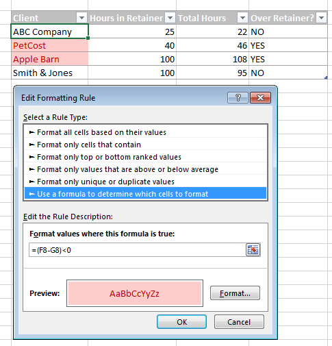
If you are used to creating complex formulas that cover all cases in one cell, it may take a little re-learning to figure out the approach for conditional formatting that works more incrementally. The best hint is to remember that you can apply multiple rules to the same cells – break up your formatting criteria into separate steps, and you’ll most likely be able to get where you need to be!
PRYOR+ 7-DAYS OF FREE TRAINING
Courses in Customer Service, Excel, HR, Leadership,
OSHA and more. No credit card. No commitment. Individuals and teams.
Combine conditional formatting with an IF statement
Syntax
=IF (logical_test, [value_if_true], [value_if_false])
But in conditional formatting, IF/THEN/ELSE syntax cannot be applied in a single rule. Conditional formatting is applied using IF/THEN logical test only. It must return TRUE for conditional formatting to be applied.
For example, if you want to apply conditional formatting using a condition that “If a cell value is greater than a set value, say 100, then format the cell as RED, else format the cell as GREEN”. So, you can see that it requires two rules to perform the conditional formatting, one for greater than 100, and one for less than 100.
You can apply more than one condition by creating more than one rule in conditional formatting. You can also use logical functions like AND and OR to create a rule set and apply conditional formatting in Excel.
Examples using conditional formatting with IF/THEN conditions
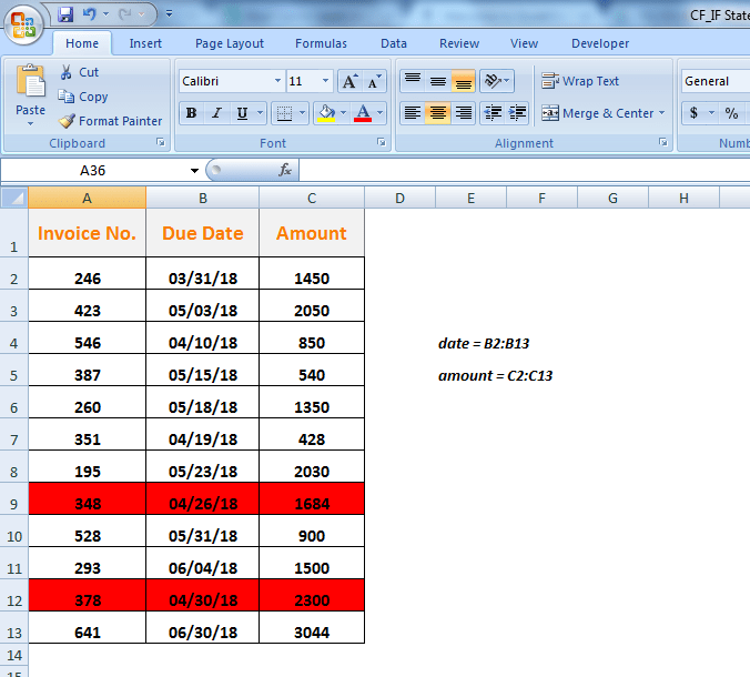
Let’s look at the scenarios to see how to use IF/THEN logical test in conditional formatting to highlight the targeted values. If you want to highlight the invoices in data range of A2:C13 which are due in the month of April, then you need to test the IF/THEN logical condition on date range in column B, if the month is equal to April, by using following custom formula in conditional formatting.=MONTH($B2)=4
First, select the data range A2:C13, then go to:
Conditional Formatting (on the Home tab) > New Rule> Use a formula to determine…> Enter the above formula in Edit Rule Description window> Choose the Format Fill to preview and press OK
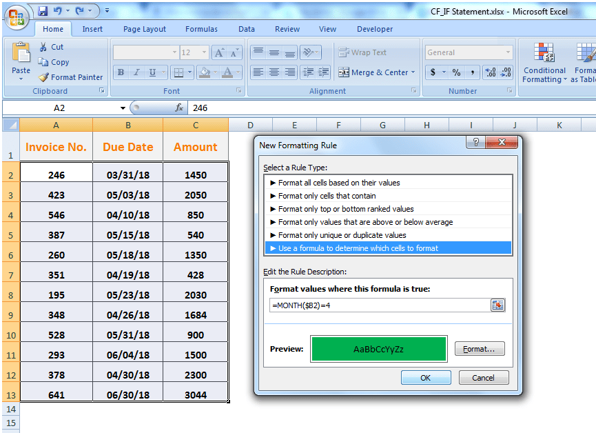
Please note that you have to fix the column by making it absolute using $ sign with it, and keep the row number free or relative to change. Hence, the formula will check each row of the specified column in the selected range, test the IF/THEN logical condition and will return TRUE and FALSE.
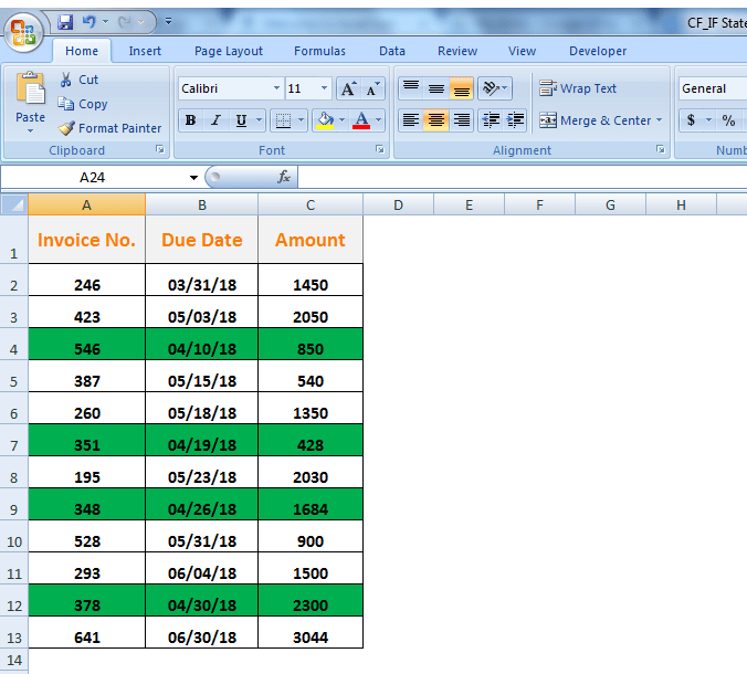
This rule will be evaluated in all active cells of locked column B one by one ignoring other cells in columns A and C. When the MONTH function in a cell of column B returns number 4 (April), the rule will return TRUE for all the active cells in that row and conditional formatting will be applied to that entire row as shown below.
Now, if you want to conditionally highlight the two largest amount invoices due in the month of April, then you can achieve this by creating a rule set based on array formula using AND, LARGE and IF statement as per the following syntax.
=AND(criteria,$C2>=LARGE (IF(criteria, values),2)) =AND(MONTH($B2)=criteria,$C2>=LARGE (IF(MONTH(date)=criteria, amount),2)) =AND(MONTH($B2)=4,$C2>=LARGE(IF(MONTH($B$2:$B$13)=4,$C$2:$C$13),2))
By applying this custom formula, you can highlight the two largest amount invoices in the month of April. LARGE with IF function will generate a series of values and compare them with each value in column C. AND function will test the logical conditions in each cell of column B and C both one by one and will return TRUE where both conditions will be met. Have a look below.
Need some additional help with Conditional Formatting or have other questions about Excel? Connect with a live Excel expert here for some 1 on 1 help. Your first session is always free.
Are you still looking for help with the Average function? View our comprehensive round-up of Average function tutorials here.
In this article we will learn how to color rows based on text criteria we use the “Conditional Formatting” option. This option is available in the “Home Tab” in the “Styles” group in Microsoft Excel.
Conditional Formatting in Excel is used to highlight the data on the basis of some criteria. It would be difficult to see various trends just for examining your Excel worksheet. Conditional Formatting in excel provides a way to visualize data and make worksheets easier to understand.
Excel Conditional Formatting allows you to apply formatting basis on the cell values such as colors, icons and data bars. For this, we will create a rule in excel Conditional Formatting based on cell value
How to write an if statement in excel?
IF function is used for logic_test and returns value on the basis of the result of the logic_test. Excel conditional formatting formula multiple conditions uses Statements like less than or equal to or greater than or equal to the value are used in IF formula
Syntax:
=IF (logical_test, [value_if_true], [value_if_false])
Let’s learn how to do conditional formatting in excel using IF function with the example.
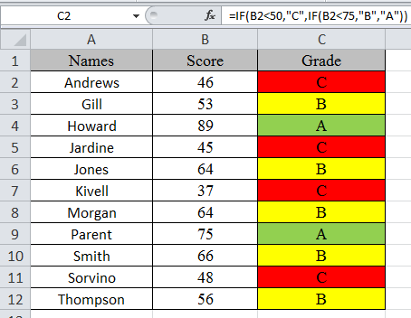
Here is a list of Names and their respective Scores.
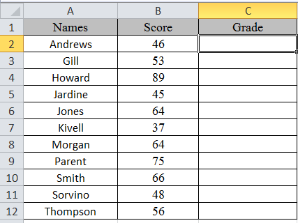
multiple if statements excel functions are used here. So, there are 3 results based on the condition. if then statements in excel is used via excel conditional formatting formula
Write the formula in C2 cell.
Formula
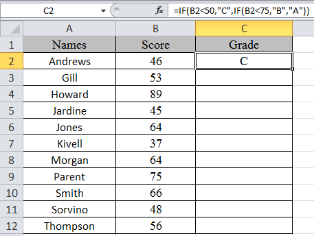
=IF(B2<50,»C»,IF(B2<75,»B»,»A»))
Explanation:
IF function only returns 2 results, one [value_if_True] and Second [value-if_False]
First IF function checks, if the score is less than 50, would get C grade, The Second IF function tests if the score is less than 75 would get B grade and the rest A grade.
Copy the formula in other cells, select the cells taking the first cell where the formula is already applied, use shortcut key Ctrl + D
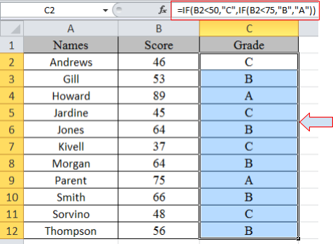
Now we will apply conditional formatting to it.
Select Home >Conditional Formatting > New Rule.
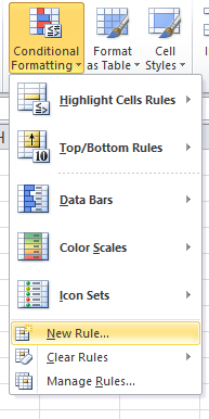
A dialog box appears
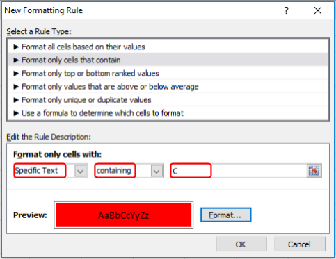
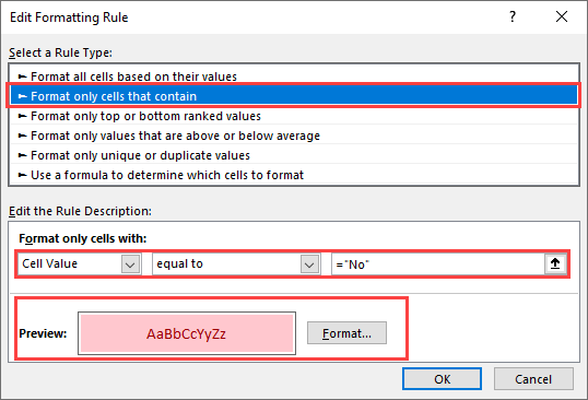
Select Format only cells that contain > Specific text in option list and write C as text to be formatted.
Fill Format with Red colour and click OK.
Now select the colour Yellow and Green for A and B respectively as done above for C.
In this article, we used IF function and Conditional formatting tool to get highlighted grade.
As you can see excel change cell color based on value of another cell using IF function and Conditional formatting tool
Hope you learned how to use conditional formatting in Excel using IF function. Explore more conditional formulas in excel here. You can perform Conditional Formatting in Excel 2016, 2013 and 2010. If you have any unresolved query regarding this article, please do mention below. We will help you.
Related Articles:
How to use the Conditional formatting based on another cell value in Excel
How to use the Conditional Formatting using VBA in Microsoft Excel
How to use the Highlight cells that contain specific text in Excel
How to Sum Multiple Columns with Condition in Excel
Popular Articles:
50 Excel Shortcut to Increase Your Productivity
How to use the VLOOKUP Function in Excel
How to use the COUNTIF function in Excel 2016
How to use the SUMIF Function in Excel
IF function is undoubtedly one of the most important functions in excel. In general, IF statements give the desired intelligence to a program so that it can make decisions based on given criteria and, most importantly, decide the program flow.
In Microsoft Excel terminology, IF statements are also called «Excel IF-Then statements». IF function evaluates a boolean/logical expression and returns one value if the expression evaluates to ‘TRUE’ and another value if the expression evaluates to ‘FALSE’.
Definition of Excel IF Function
According to Microsoft Excel, IF function is defined as a formula which «checks whether a condition is met, returns one value if true and another value if false».
Syntax
Syntax of IF function in Excel is as follows:
=IF(logic_test, [value_if_true], [value_if_false])
'logic_test' (required argument) – Refers to the boolean expression or logical expression that needs to be evaluated.'value_if_true' (optional argument) – Refers to the value that will be returned by the IF function if the 'logic_test' evaluates to TRUE.'value_if_false' (optional argument) – Refers to the value that will be returned by the IF function if the 'logic_test' evaluates to FALSE.

Important Characteristics of IF Function in Excel
- To use the IF function, you need to provide the
'logic_test'or conditional statement mandatorily. - The arguments
'value_if_true'and'value_if_false'are optional, but you need to provide at least one of them. - The result of the IF statement can only be any one of the two given values (either it will be
'value_if_true'or'value_if_false'). Both values cannot be returned at the same time. - IF function throws a ‘#Name?’ error if the
'logic_test'or boolean expression you are trying to evaluate is invalid. - Nesting of IF statements is possible, but Excel only allows this to 64 levels. Nesting of IF statement means using one if statement within another.
Comparison Operators That Can Be Used With IF Statements
Following comparison operators can be used within the 'logic_test' argument of the IF function:
- = (equal to)
- <> (not equal to)
- < (less than)
- > (greater than)
- >= (greater than or equal to)
- <= (less than or equal to)
- Apart from these, you can also use any other function that returns a boolean result (either ‘true’ or ‘false’). For example – ISBLANK, ISERROR, ISEVEN, ISODD, etc
Now, let’s see some simple examples to use these comparison operators within the IF Function:
Simple Examples of Excel IF Statement
Now, let’s try to see a simple example of the Excel IF function:
Example 1: Using ‘equal to’ comparison operator within the IF function
In this example, we have a list of colors, and we aim to find the ‘Blue’ color. If we are able to find the ‘Blue’ color, then in the adjacent cell, we need to assign a ‘Yes’; otherwise, assign a ‘No’.

So, the formula would be:
=IF(A2="Blue", "No", "Yes")
This suggests that if the value present in cell A2 is ‘Blue’, then return a ‘Yes’; otherwise, return a ‘No’.
If we drag this formula down to all the rows, we will find that it returns ‘Yes’ for the cells with the value ‘Blue’ for all others; it would result in ‘No’.
Example 2: Using ‘not equal to’ comparison operator within the IF function.
Let’s take example 1, and understand how we can reverse the logic and use a ‘not equal to’ operator to construct the formula so that it still results in ‘Yes’ for ‘Blue’ color and ‘No’ for any other text.

So the formula would be:
=IF(A2<>"Blue", "No", "Yes")
This suggests that if the value at A2 is not equal to ‘Blue’, then return a ‘No’; otherwise, return a ‘Yes’.
When dragged down to all the below rows, this formula would find all the cells (from A2 to A8) where the value is not ‘Blue’ and marks a ‘No’ against them. Otherwise, it marks a ‘Yes’ in the adjacent cells.
Example 3: Using ‘less than’ operator within the IF function.
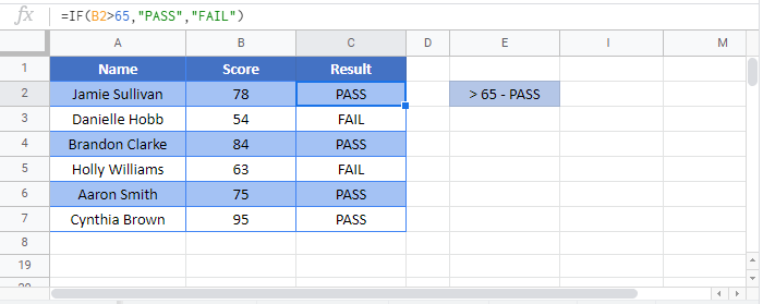
In this example, we have scores of some students, along with their names. We want to assign either «Pass» or «Fail» against each student in the result column.

Based on our criteria, the passing score is 50 or more.
For this, we can use the IF function as:
=IF(B2<50,"Fail","Pass")
This suggests that if the value at B2, i.e., 37, is less than 50, then return «Fail»; otherwise, return «Pass».
As 37 is less than 50 so the result will be «Fail».
We can drag the above-given formula for the rest of the cells below and the result would be correct.
Example 4: Using ‘greater than or equal to’ operator within the IF statement.
Let’s take example 3 and see how we can reverse the logic and use a ‘greater than or equal to’ operator to construct the formula so that it still results in ‘Pass’ for scores of 50 or more and ‘Fail’ for all the other scores.

For this, we can use the Excel IF function as:
=IF(B2>=50,"Pass","Fail")
This suggests that if the value at B2, i.e., 37 is greater than or equal to 50, then return «Pass»; otherwise, return «Fail».
As 37 not greater than or equal to 50 so the result will be «Fail».
When dragged down for the rest of the cells below, this formula would assign the correct result in the adjacent rows.
Example 5: Using ‘greater than’ operator within the IF statement.
In this example, we have a small online store that gives a discount to its customers based on the amount they spend. If a customer spends $50 or more, he is applicable for a 5% discount; otherwise, no discounts are offered.

To find whether a discount is offered or not, we can use the following excel formula:
=IF(B2>50,"5% Discount","No Discount")
This translates to – If the value at B2 cell is greater than 50, assign a text «5% Discount» otherwise, assign a text «No Discount» against the customer.
In the first case, as 23 is not greater than 50, the output will be «No Discount».
We can drag the above-given formula for the rest of the cells below are the result would be correct.
Example 6: Using ‘less than or equal to’ operator within the IF statement.
Let’s take example 5 and see how we can reverse the logic and use a ‘less than or equal to’ operator to construct the formula so that it still results in a ‘5% Discount’ for all customers whose total spend exceeds $50 and ‘No Discount’ for all the other customers.

For this, we can use the IF-then statement as:
=IF(B2<=50,"No Discount","5% Discount")
This means that if the value at B2, i.e., 23, is less than or equal to 50, then return «No Discount»; otherwise, return «5% Discount».
As 23 is less than or equal to 50 so the result will be «No Discount».
When dragged down for the rest of the cells below, this formula would assign the correct result in the adjacent rows.
Example 7: Using an Excel Logical Function within the IF formula in Excel.
In this example, let’s suppose we have a list of numbers, and we have to mark Even and Odd numbers. We can do this using the IF condition and the ISEVEN or ISODD inbuilt functions provided by Microsoft Excel.
ISEVEN function returns ‘true’ if the number passed to it is even; otherwise, it returns a ‘false’. Similarly, ISODD function return ‘true’ if the number passed to it is odd; otherwise, it returns a ‘false’.

For this, we can use the IF-then statement as:
=IF(ISEVEN(A2),"Even","Odd")
This means that – If the value at A2 cell is an even number, then the result would be «Even»; otherwise, the result would be «Odd».
Alternatively, the above logic can also be written using the ISODD function along with the IF statement as:
=IF(ISODD(A2),"Odd","Even")
This means that – If the value at A2 cell is an odd number, then the result would be «Odd»; otherwise, the result would be «Even».
Example 8: Using the Excel IF function to return another formula a result.
In this example, we have Employee Data from a company. The company comes up with a simple way to reward its loyal employees. They decide to give the employees an annual bonus based on the years spent by the employee within the organization.
Employees with experience of more than 5 years are given 10% of annual salary as a bonus whereas everyone else gets a 5% of annual salary as a bonus.

For this, the excel formula would be:
=IF(B2>5,C2*10%,C2*5%)
This means that – if the value at B2 (experience column) is greater than 5, then return a result by calculating 10% of C2 (annual salary column). However, if the logic test is evaluated to false, then return the result by calculating 5% of C2 (annual salary column)
Use Of AND & OR Functions or Logical Operators with Excel IF Statement
Excel IF Statement can also be used along with the other functions like AND, OR, NOT for analyzing complex logic. These functions (AND, OR & NOT) are called logical operators as they are used for connecting two or more logical expressions.
AND Function– AND function returns true when all the conditions inside the AND function evaluate to true. The syntax of AND Function in Excel is:
=AND(Logic1, Logic2, logic_n)
OR Function– OR function returns true when any one of the conditions inside the OR function evaluates to true. The syntax of OR Function in Excel is:
=OR(Logic1, Logic2, logic_n)
Example 9: Using the IF function along with AND Function.
In this example, we have Math and science test scores of some students, and we want to assign a ‘Pass’ or ‘Fail’ value against the students based on their scores.
Passing criteria: Students have to get more than 50 marks in Math and more than 70 marks in science to pass the test.

Based on the above conditions, the formula would be:
=IF(AND(B2>50,C2>70),"Pass","Fail")
The formula translates to – if the value at B2 (Math score) is greater than 50 and the value at C2 (Science Score) is greater than 70, then assign the value «Pass»; otherwise, assign the value «Fail».
Example 10: Using the IF function along with OR Function.
In this example, we have two test scores of some students, and we want to assign a ‘Pass’ or ‘Fail’ value against the students based on their scores.
Passing criteria: Students have to clear either one of the two tests with more than 50 marks.

Based on the above conditions, the formula would be:
=IF(OR(B2>50,C2>50),"Pass","Fail")
The formula translates to – if either the value at B2 (Test 1 score) is greater than 50, OR the value at C2 (Test 2 Score) is greater than 50, then assign the value «Pass»; otherwise, assign the value «Fail».
Recommended Reading: Excel NOT Function
Nested IF Statements
When used alone, IF formula can only result in two outcomes, i.e., True or False. But there are many cases when we want to test multiple outcomes with IF statement.
In such cases, nesting two or more IF Then statements one inside another can be convenient in writing formulas.
Syntax:
The syntax of the Nested IF Then statements is as follows:
=IF(condition_1,value_if_true_1,IF(condition_2,value_if_true_2,value_if_false_2))
'condition_1' – Refers to the first logical test or conditional expression that needs to be evaluated by the outer IF function.'value_if_true_1' – Refers to the value that will be returned by the outer IF function if the 'condition_1' evaluates to TRUE.'condition_2' – Refers to the second logical test or conditional expression that needs to be evaluated by the inner IF function.'value_if_true_2' – Refers to the value that will be returned by the inner IF function if the 'condition_2' evaluates to TRUE.'value_if_false_2' – Refers to the value that will be returned by the inner IF function if the 'condition_2' evaluates to FALSE.
The above syntax translates to this:
IF Condition1 = true THEN value_if_true1 'If Condition1 is true
ELSE IF Condition2 = true THEN value_if_true2 'Elseif Clause Condition2 is true
ELSE value_if_false2 'If both conditions are false
END IF 'End of IF Statement
As we can see, Nested formulas can quickly become complicated so, let’s try to understand how nesting of the IF statement works with an example.
Recommended Reading: VBA Select Case Statement
Example 11: Nested IF Statements
In this example, we have a list of countries and their average temperatures in degree Celsius for the month of January. Our goal is to categorize the country based on the temperature range as follows:
Criteria: Temperatures below 20 °C should be marked as «Below Room Temperature», temperatures between 20°C to 25°C should be classified as «Normal Room Temperature», whereas any temperature over 25°C should be marked as «Above Room Temperature».

Based on the above conditions, the formula would be:
=IF(B2<20,"Below Room Temperature",IF(AND(B2>=20,B2<=25),"Normal Room Temperature", "Above Room Temperature"))
The formula translates to – if the value at B2 is less than 20, then the text «Below Room Temperature» is returned from the outer IF block. However, if the value at B2 is greater than or equal to 20, then the inner IF block is evaluated.
Inside the inner IF block, the value at B2 is checked. If the value at B2 is greater than or equal to 20 and less than or equal to 25. Then the inner IF block returns the text «Normal Room Temperature».
However, if the condition inside the inner IF block also evaluates to ‘false’ that means the value at B2 is greater than 25, so the result will be «Above Room Temperature».
Recommended Reading: SWITCH Function in Excel
Partial Matching or Wildcards with IF Function
Although IF function itself doesn’t accept any wildcard characters like (* or ?) while performing the logic test, thankfully, there are ways to perform partial matching and wildcard searches with the IF function.
To perform partial matching inside the IF function, we can use the FIND (case sensitive) or SEARCH (case insensitive) functions.
Let’s have a look at this with some examples.
Example 12: Using FIND and SEARCH functions inside the IF statement
In this example, we have a list of customers, and we need to find all the customers whose last name is «Flynn». If the customer name contains the text «Flynn», then we need to assign a text «Found» against their names. Otherwise, we need to assign a text «Not Found».

For this, we can make use of the FIND function within the IF function as:
=IF(ISNUMBER(FIND("Flynn",A2)),"Found","Not Found")
Using the FIND function, we perform a case-sensitive search of the text «Flynn» within the customer name column. If the FIND function is able to find the text «Flynn», it returns a number signifying the position where it found the text.
If the number returned by the FIND function is valid, the ISNUMBER Function returns a value true. Else, it returns false. Based on the ISNUMBER function’s output, the logic test is performed and the appropriate value «Found» or «Not Found» is assigned.
Note: It should be noted that the FIND function performs a case-sensitive search.
This means in the above example if the customer name is entered in lower case (like «sean flynn» then the above function would return not found against them.
To perform a case-insensitive search, we can replace the find function with the search function, and the rest of the formula would be the same.
=IF(ISNUMBER(SEARCH("Flynn",A2)),"Found","Not Found")
Example 13: Using SEARCH function inside the Excel IF formula with wildcard operators
In this example, we have the same customer list from example 12, and we need to find all the customers whose name contains «M». If the customer name contains the alphabet «M», we need to assign a text «M Found» against their names. Otherwise, we need to assign a text «M Not Found».

For this, we can use the SEARCH function with a wildcard ‘*’ operator inside the IF function as:
=IF(ISNUMBER(SEARCH("M*",A2)),"M Found","M Not Found")
For more details on Search Function and wildcard, operators check out this article – Search Function In Excel
Some Practical Examples of using the IF function
Now, let’s have a look at some more practical examples of the Excel IF Function.
Example 14: Using Excel IF function with dates.
In this example, we have a task list along with the task due dates. Our goal is to show results based on the task due date.
If the task due date was in the past, we need to show «Was due {1,2,3..} day(s) back», if the task due date is today’s date, we need to show «Today» and similarly, if the task due date is in the future then we need to show «Due in {1,2,3..} day(s)»

In Microsoft Excel, we can do this with the help of the IF-then statement and TODAY function, as shown below:
=IF(B2=TODAY(),"Today", IF(B2>TODAY(),CONCAT("Due in ",B2-TODAY()," day(s)"), CONCAT("Was due ",TODAY()-B2," day(s) back")))
This means that – compare the date present in cell B2 if the date is equal to today’s date show the text «Today». If the date in cell B2 is not equal to today’s date, then the inner IF block checks if the date in B2 is greater than today’s date. If the date in cell B2 is greater than today’s date, that means the date is in the future, so show the text «Due in {1,2,3…} days».
However, if the date in cell B2 is not greater than today’s date, that means the date was in the past; in such a case, show the text «Was due {1,2,3..} day(s) back».
You can also go a step further and apply conditional formatting on the range and highlight all the cells with the text «Today!». This will help you to clearly see
Example 15: Use an IF function-based formula to find blank cells in excel.
In this example, we will use the IF function to find the blank cells in Microsoft Excel. We have a list of customers, and in between the list, some of the cells are blank. We aim to find the blank cells and add the text «blank call found!» against them.

We can do this with the help of the IF function along with the ISBLANK function. The ISBLANK function returns a true if the cell reference passed to it is blank. Otherwise, the ISBLANK function returns false.
Let’s see the formula –
=IF(ISBLANK(A2), "Blank cell found!"," ")
This means that – If the cell at A2 is blank, then the resultant text should be «Blank cell found!», however, if the cell at A2 is not blank, then don’t show any text.
Example 16: Use the Excel IF statement to show symbolic results (instead of textual results).
In this example, we have a list of sales employees of a company along with the number of products sold by the employees in the current month. We want to show an upward arrow symbol (↑) if the employee has done more than 50 sales and a downward arrow symbol (↓) if the employee has made less than 50 sales.

To do this, we can use the formula:
=IF(B2>50,$G$6,$G$8)
This implies – If the value at B2 is greater than 50, then, as a result, show the content in cell G6 (cell containing upward arrow) and otherwise show the content at G8 (cell containing downward arrow)
If you wonder about the ‘$’ signs used in the formula, you can check out this post – Excel Absolute References. These ‘$’ symbols are used for making excel cell references absolute.
Recommended Reading: CHOOSE Function in Excel
IFS Function In Excel:
IFS Function in Microsoft Excel is a great alternative to nested IF Statements. It is very similar to a switch statement. The IFS function evaluates multiple conditions passed to it and returns the value corresponding to the first condition that evaluates to true.
IFS function is a lot simple to write and read than nested IF statements. IFS function is available in Office 2019 and higher versions.
Syntax for IFS function:
=IFS (test1, value1, [test2, value2], ...)
'test1' (required argument) – Refers to the first logical test that needs to be evaluated.
'value1' (required argument) – Refers to the result to be returned when 'test1'evaluates to TRUE.
'test2' (optional argument) – Refers to the second logical test that needs to be evaluated
'value2' (optional argument) – Refers to the result to be returned when 'test2'evaluates to TRUE.
Example 17: Using IFS function in Excel
In this example, we have a list of students, along with their scores, and we need to assign a grade to the students based on the scores.
The grading criteria is as follows – Grade A for a score of 90 or more, Grade B for a score between 80 to 89.99, Grade C for a score between 70 to 79.99, Grade D for a score between 60 to 69.99, Grade E for a score between 60 to 59.99, Grade F for a score lower than 50.

Let’s see how easily write such a complicated formula with the IFS function:
=IFS(B2 >= 90,"A",B2 >= 80,"B",B2 >= 70,"C",B2 >= 60,"D",B2 >= 50,"E",B2 < 50,"F")
This implies that – If B2 is greater than or equal to 90, return A. Else if B2 is greater than or equal to 80, return B. Else if B2 is greater than or equal to 70, return C. Else if B2 is greater than or equal to 60, return D. Else if B2 is greater than or equal to 50, return E. Else if B2 is less than 50, return F.
If you would try to write the same formula using nested IF statements, see how long and complicated it becomes:
=IF(B2 >= 90,"A",IF(B2 >= 80, "B",IF(B2 >= 70, "C",IF(B2 >= 60, "D",IF(B2 >= 50, "E",IF(B2 < 50, "F"))))))
So, this was all about the IF function in excel. If you want to learn more about IF function, I would recommend you to go through this article – VBA IF Statement With Examples
The logical IF statement in Excel is used for the recording of certain conditions. It compares the number and / or text, function, etc. of the formula when the values correspond to the set parameters, and then there is one record, when do not respond — another.
Logic functions — it is a very simple and effective tool that is often used in practice. Let us consider it in details by examples.
The syntax of the function «IF» with one condition
The operation syntax in Excel is the structure of the functions necessary for its operation data.
=IF(boolean;value_if_TRUE;value_if_FALSE)
Let us consider the function syntax:
- Boolean – what the operator checks (text or numeric data cell).
- Value_if_TRUE – what will appear in the cell when the text or numbers correspond to a predetermined condition (true).
- Value_if_FALSE – what appears in the box when the text or the number does not meet the predetermined condition (false).
Example:

Logical IF functions.
The operator checks the A1 cell and compares it to 20. This is a «Boolean». When the contents of the column is more than 20, there is a true legend «greater 20». In the other case it’s «less or equal 20».
Attention! The words in the formula need to be quoted. For Excel to understand that you want to display text values.
Here is one more example. To gain admission to the exam, a group of students must successfully pass a test. The results are listed in a table with columns: a list of students, a credit, an exam.

The statement IF should check not the digital data type but the text. Therefore, we prescribed in the formula В2= «done» We take the quotes for the program to recognize the text correctly.
The function IF in Excel with multiple conditions
Usually one condition for the logic function is not enough. If you need to consider several options for decision-making, spread operators’ IF into each other. Thus, we get several functions IF in Excel.
The syntax is as follows:
Here the operator checks the two parameters. If the first condition is true, the formula returns the first argument is the truth. False — the operator checks the second condition.
Examples of a few conditions of the function IF in Excel:

It’s a table for the analysis of the progress. The student received 5 points:
- А – excellent;
- В – above average or superior work;
- C – satisfactory;
- D – a passing grade;
- E – completely unsatisfactory.
IF statement checks two conditions: the equality of value in the cells.

In this example, we have added a third condition, which implies the presence of another report card and «twos». The principle of the operator is the same.
Enhanced functionality with the help of the operators «AND» and «OR»
When you need to check out a few of the true conditions you use the function И. The point is: IF A = 1 AND A = 2 THEN meaning в ELSE meaning с.
OR function checks the condition 1 or condition 2. As soon as at least one condition is true, the result is true. The point is: IF A = 1 OR A = 2 THEN value B ELSE value C.
Functions AND & OR can check up to 30 conditions.
An example of using the operator AND:

It’s the example of using the logical operator OR.

How to compare data in two tables
Users often need to compare the two spreadsheets in an Excel to match. Examples of the «life»: compare the prices of goods in different bringing, to compare balances (accounting reports) in a few months, the progress of pupils (students) of different classes, in different quarters, etc.
To compare the two tables in Excel, you can use the COUNTIFS statement. Consider the order of application functions.
For example, consider the two tables with the specifications of various food processors. We planned allocation of color differences. This problem in Excel solves the conditional formatting.
Baseline data (tables, which will work with):

Select the first table. Conditional Formatting — create a rule — use a formula to determine the formatted cells:

In the formula bar write: = COUNTIFS (comparable range; first cell of first table)=0. Comparing range is in the second table.
To drive the formula into the range, just select it first cell and the last. «= 0» means the search for the exact command (not approximate) values.
Choose the format and establish what changes in the cell formula in compliance. It’s better to do a color fill.
Select the second table. Conditional Formatting — create a rule — use the formula. Use the same operator (COUNTIFS). For the second table formula:
Download all examples in Excel

Now it is easy to compare the characteristics of the data in the table.
This tutorial demonstrates how to use the IF Function in Excel and Google Sheets to create If Then Statements.
IF Function Overview
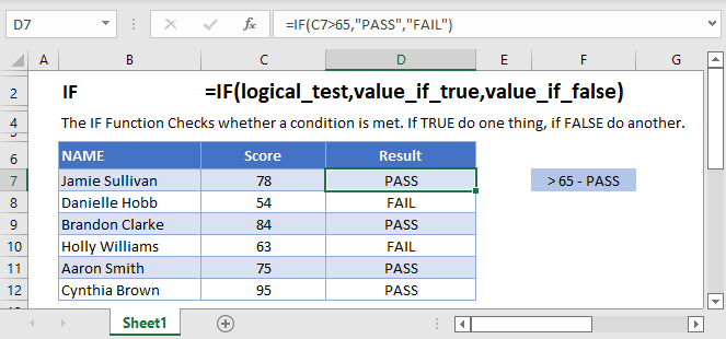
The IF Function Checks whether a condition is met. If TRUE do one thing, if FALSE do another.
How to Use the IF Function
Here’s a very basic example so you can see what I mean. Try typing the following into Excel:
=IF( 2 + 2 = 4,"It’s true", "It’s false!")Since 2 + 2 does in fact equal 4, Excel will return “It’s true!”. If we used this:
=IF( 2 + 2 = 5,"It’s true", "It’s false!")Now Excel will return “It’s false!”, because 2 + 2 does not equal 5.
Here’s how you might use the IF statement in a spreadsheet.
=IF(C4-D4>0,C4-D4,0)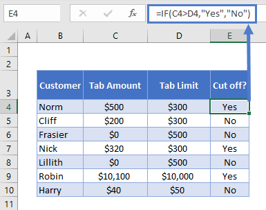
You run a sports bar and you set individual tab limits for different customers. You’ve set up this spreadsheet to check if each customer is over their limit, in which case you’ll cut them off until they pay their tab.
You check if C4-D4 (their current tab amount minus their limit), is greater than 0. This is your logical test. If this is true, IF returns “Yes” – you should cut them off. If this is false, IF returns “No” – you let them keep drinking.
What can IF Return?
Above we returned a text string, “Yes” or “No”. But you can also return numbers, or even other formulas.
Let’s say some of your customers are running up big tabs. To discourage this, you’re going to start charging interest on customers who go over their limit.
You can use IF for that:
=IF(C4>D4,C4*0.03,0)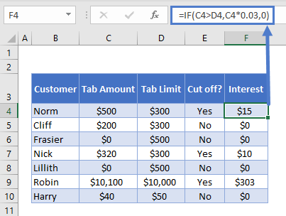
If the tab is higher than the limit, return the tab multiplied by 0.03, which returns 3% of the tab. Otherwise, return 0: they aren’t over their tab, so you won’t charge interest.
Using IF with AND
You can combine IF with Excel’s AND Function to test more than one condition. Excel will only return TRUE if ALL of the tests are true.
So, you implemented your interest rate. But some of your regulars are complaining. They’ve always paid their tabs in the past, why are you cracking down on them now? You come up with a solution: you won’t charge interest to certain trusted customers.
You make a new column to your spreadsheet to identify trusted customers, and update your IF statement with an AND function:
=IF(AND(C4>D4, F4="No"),C4*0.03,0)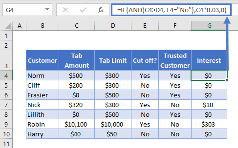
Let’s look at the AND part separately:
AND(C4>D4, F4="No")Note the two conditions:
- C4>D4: checking if they’re over their tab limit, as before
- F4=”No”: this is the new bit, checking if they are not a trusted customer
So now we only return the interest rate if the customer is over their tab, AND we have “No” in the trusted customer column. Your regulars are happy again.
Using IF with OR
The OR Function allows you to test more than one condition, returning TRUE if any conditions are met.
Maybe customers being over their tab is not the only reason you’d cut them off. Maybe you give some people a temporary ban for other reasons, gambling on the premises perhaps.
So you add a new column to identify banned customers, and update your “Cut off?” column with an OR test:
=IF(OR(C4>D4,E4="Yes"),"Yes","No")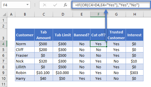
Looking just at the OR part:
OR(C4>D4,E4="Yes")There are two conditions:
- C4>D4: checking if they’re over their tab limit
- F4=”Yes”: the new part, checking if they are currently banned
This will evaluate to true if they are over their tab, or if there is a “Yes” in column E. As you can see, Harry is cut off now, even though he’s not over his tab limit.
Using IF with XOR
The XOR Function returns TRUE if only one condition is met. If more than one condition is met (or not conditions are met). It returns FALSE.
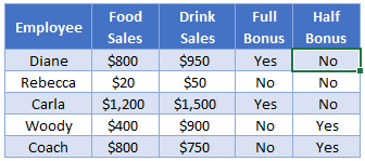
An example might make this clearer. Imagine you want to start giving monthly bonuses to your staff :
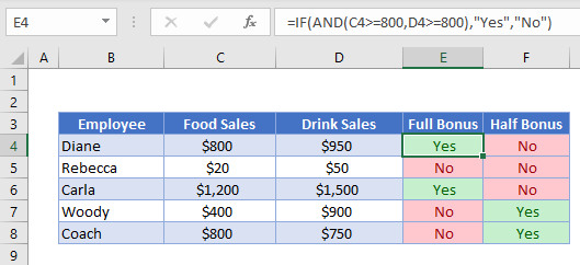
- If they sell over $800 in food, or over $800 in drinks, you’ll give them a half bonus
- If they sell over $800 in both, you’ll give them a full bonus
- If they sell under $800 in both, they don’t get any bonus.
You already know how to work out if they get the full bonus. You’d just use IF with AND, as described earlier.
=IF(AND(C4>800,D4>800),"Yes","No")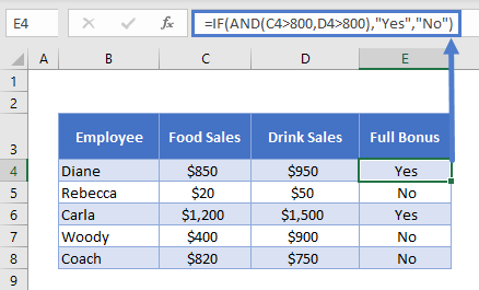
But how would you work out who gets the half bonus? That’s where XOR comes in:
=IF(XOR(C4>=800,D4>=800),"Yes","No")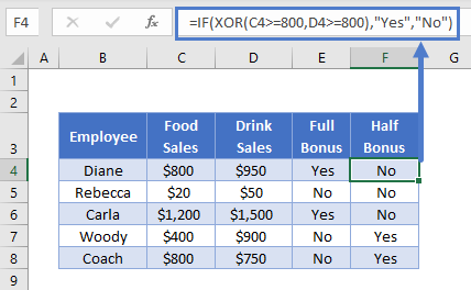
As you can see, Woody’s drink sales were over $800, but not food sales. So he gets the half bonus. The reverse is true for Coach. Diane and Carla sold more than $800 for both, so they don’t get a half bonus (both arguments are TRUE), and Rebecca made under the threshold for both (both arguments FALSE), so the formula again returns “No”.
Using IF with NOT
The NOT Function reverses the outcome of a logical test. In other words, it checks whether a condition has not been met.
You can use it with IF like this:
=IF(AND(C3>=1985,NOT(D3="Steven Spielberg")),"Watch", "Don’t Watch")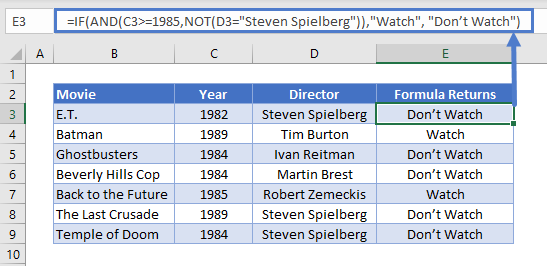
Here we have a table with data on some 1980s movies. We want to identify movies released on or after 1985, that were not directed by Steven Spielberg.
Because NOT is nested within an AND Function, Excel will evaluate that first. It will then use the result as part of the AND.
Nested IF Statements
You can also return an IF statement within your IF statement. This enables you to make more complex calculations.
Let’s go back to our customers table. Imagine you want to classify customers based on their debt level to you:
- $0: None
- Up to $500: Low
- $500 to $1000: Medium
- Over $1000: High
You can do this by “nesting” IF statements:
=IF(C4=0,"None",IF(C4<=500,"Low",IF(C4<=1000,"Medium",IF(C4>1000,"High"))))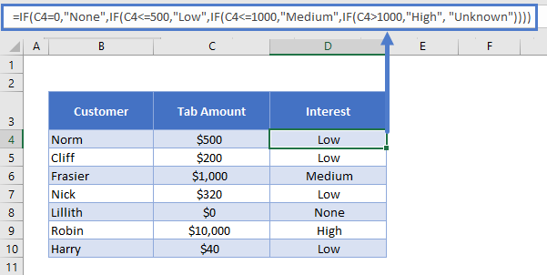
It’s easier to understand if you put the IF statements on separate lines (ALT + ENTER on Windows, CTRL + COMMAND + ENTER on Macs):
=
IF(C4=0,"None",
IF(C4<=500,"Low",
IF(C4<=1000,"Medium",
IF(C4>1000,"High", "Unknown"))))
IF C4 is 0, we return “None”. Otherwise, we move to the next IF statement. IF C4 is equal to or less than 500, we return “Low”. Otherwise, we move on to the next IF statement… and so on.
Simplifying Complex IF Statements with Helper Columns
If you have multiple nested IF statements, and you’re throwing in logic functions too, your formulas can become very hard to read, test, and update.
This is especially important to keep in mind if other people will be using the spreadsheet. What makes sense in your head, might not be so obvious to others.
Helper columns are a great way around this issue.
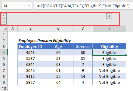
You’re an analyst in the finance department of a large corporation. You’ve been asked to create a spreadsheet that checks whether each employee is eligible for the company pension.
Here’s the criteria:
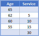
So if you’re under the age of 55, you need to have 30 years’ service under your belt to be eligible. If you’re aged 55 to 59, you need 15 years’ service. And so on, up to age 65, where you’re eligible no matter how long you’ve worked there.
You could use a single, complex IF statement to solve this problem:
=IF(OR(F4>=65,AND(F4>=62,G4>=5),AND(F4>=60,G4>=10),AND(F4>=55,G4>=15),G4>30),"Eligible", "Not Eligible")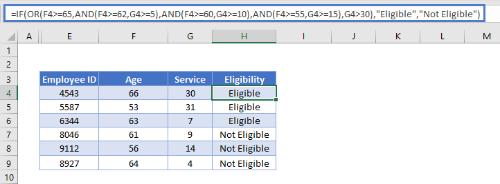
Whew! Kinda hard to get your head around that, isn’t it?
A better approach might be to use helper columns. We have five logical tests here, corresponding to each row in the criteria table. This is easier to see if we add line breaks to the formula, as we discussed earlier:
=IF(
OR(
F4>=65,
AND(F4>=62,G4>=5),
AND(F4>=60,G4>=10),
AND(F4>=55,G4>=15),
G4>30
),"Eligible","Not Eligible")
So, we can split these five tests into separate columns, and then simply check whether any one of them is true:
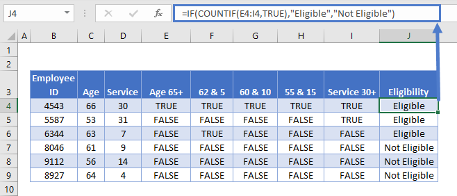
Each column in the table from E to I holds each of our criteria separately. Then in J4 we have the following formula:
=IF(COUNTIF(E4:I4,TRUE),"Eligible","Not Eligible")Here we have an IF statement, and the logical test uses COUNTIF to count the number of cells within E4:I4 that contain TRUE.
If COUNTIF doesn’t find a TRUE value, it will return 0, which IF interprets as FALSE, so the IF returns “Not Eligible”.
If COUNTIF does find any TRUE values, it will return the number of them. IF interprets any number other than 0 as TRUE, so it returns “Eligible”.
Splitting out the logical tests in this way makes the formula easier to read, and if something’s going wrong with it, it’s much easier to spot where the mistake is.
Using Grouping to Hide Helper Columns
Helper columns make the formula easier to manage, but once you’ve got them in place and you know they are working correctly, they often just take up space on your spreadsheet without adding any useful information.
You could hide the columns, but this can lead to problems because hidden columns are hard to detect, unless you look closely at the column headers.
A better option is grouping.
Select the columns you want to group, in our case E:I. Then press ALT + SHIFT + RIGHT ARROW on Windows, or COMMAND + SHIFT + K on Mac. You can also go to the “Data” tab on the ribbon and select “Group” from the “Outline” section.
You’ll see the group displayed above the column headers, like this:
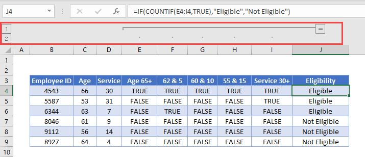
Then simply press the “-“ button to hide the columns:
The IFS Function
Nested IF statements are very useful when you need to perform more complex logical comparisons, and you need to do it in one cell. However, they can get complicated as they get longer, and they can be hard to read and update on your screen.
From Excel 2019 and Excel 365, Microsoft introduced another function, the IFS Function, to help make this a bit easier to manage. The nested IF example above could be achieved with IFS like this:
=IFS(
C4=0,"None",
C4<=500,"Low",
C4<=1000,"Medium",
C4>1000,"High",
TRUE, "Unknown",
)
You can read all about it on the main page for the Excel IFS Function <<link>>.
Using IF with Conditional Formatting
Excel’s Conditional Formatting feature enables you to format a cell in different ways depending on its contents. Since the IF returns different values based on our logical test, we might want to use Conditional Formatting with the IF Function to make these different values easier to see.
So let’s go back to our staff bonus table from earlier.
We’re returning “Yes” or “No” depending on what bonus we want to give. This tells us what we need to know, but the information doesn’t jump out at us. Let’s try to fix that.
Here’s how you’d do it:
- Select the cell range containing your IF statements. In our case that’s E4:F8.
- Click “Conditional Formatting” on the “Styles” section of the “Home” tab on the ribbon.
- Click “Highlight Cells Rules” and then “Equal to”.
- Type “Yes” (or whatever return value you need) into the first box, and then choose the formatting you want from the second box. (I’ll choose green for this).
- Repeat for all your return values (I’ll also set “No” values to red)
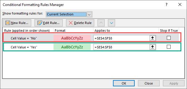
Here’s the result:
Using IF in Array Formulas
An array is a range of values, and in Excel arrays are represented as comma separated values enclosed in braces, such as:
{1,2,3,4,5}The beauty of arrays, is that they enable you to perform a calculation on each value in the range, and then return the result. For example, the SUMPRODUCT Function takes two arrays, multiplies them together, and sums the results.
So this formula:
=SUMPRODUCT({1,2,3},{4,5,6})…returns 32. Why? Let’s work it through:
1 * 4 = 4
2 * 5 = 10
3 * 6 = 18

4 + 10 + 18 = 32
We can bring an IF statement into this picture, so that each of these multiplications only happens if a logical test returns true.
For example, take this data:
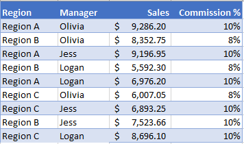
If you wanted to calculate the total commission for each sales manager, you’d use the following:
=SUMPRODUCT(IF($C$2:$C$10=$G2,$D$2:$D$10*$E$2:$E$10))Note: In Excel 2019 and earlier, you have to press CTRL + SHIFT + ENTER to turn this into an array formula.
We’d end up with something like this:
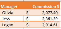
Breaking this down, the “Manager” column is column C, and in this example, Olivia’s name is in G2.
So the logical test is:
$C$2:$C$10=$G2In English, if the name in column C is equal to what’s in G2 (“Olivia”), DO multiply the values in columns D and E for that row. Otherwise, don’t multiply them. Then, sum all the results.
You can learn more about this formula on the main page for the SUMPRODUCT IF Formula.
IF in Google Sheets
The IF Function works exactly the same in Google Sheets as in Excel:
VBA IF Statements
You can also use If Statements in VBA. Click the link to learn more, but here is a simple example:
Sub Test_IF ()

If Range("a1").Value < 0 then
  Range("b1").Value = "Negative"
End If

End Sub
This code will test if a cell value is negative. If so, it will write “negative” in the next cell.
The IF function runs a logical test and returns one value for a TRUE result, and another value for a FALSE result. The result from IF can be a value, a cell reference, or even another formula. By combining the IF function with other logical functions like AND and OR, you can test more than one condition at a time.
Syntax
The generic syntax for the IF function looks like this:
=IF(logical_test,[value_if_true],[value_if_false])The first argument, logical_test, is typically an expression that returns either TRUE or FALSE. The second argument, value_if_true, is the value to return when logical_test is TRUE. The last argument, value_if_false, is the value to return when logical_test is FALSE. Both value_if_true and value_if_false are optional, but you must provide one or the other. For example, if cell A1 contains 80, then:
=IF(A1>75,TRUE) // returns TRUE
=IF(A1>75,"OK") // returns "OK"
=IF(A1>85,"OK") // returns FALSE
=IF(A1>75,10,0) // returns 10
=IF(A1>85,10,0) // returns 0
=IF(A1>75,"Yes","No") // returns "Yes"
=IF(A1>85,"Yes","No") // returns "No"
Notice that text values like «OK», «Yes», «No», etc. must be enclosed in double quotes («»). However, numeric values should not be enclosed in quotes.
Logical tests
The IF function supports logical operators (>,<,<>,=) when creating logical tests. Most commonly, the logical_test in IF is a complete logical expression that will evaluate to TRUE or FALSE. The table below shows some common examples:
| Goal | Logical test |
|---|---|
| If A1 is greater than 75 | A1>75 |
| If A1 equals 100 | A1=100 |
| If A1 is less than or equal to 100 | A1<=100 |
| If A1 equals «Red» | A1=»red» |
| If A1 is not equal to «Red» | A1<>»red» |
| If A1 is less than B1 | A1<B1 |
| If A1 is empty | A1=»» |
| If A1 is not empty | A1<>»» |
| If A1 is less than current date | A1<TODAY() |
Notice text values must be enclosed in double quotes («»), but numbers do not. The IF function does not support wildcards, but you can combine IF with COUNTIF to get basic wildcard functionality. To test for substrings in a cell, you can use the IF function with the SEARCH function.
Pass or Fail example
In the worksheet shown above, we want to assign either «Pass» or «Fail» based on a test score. A passing score is 70 or higher. The formula in D6, copied down, is:
=IF(C5>=70,"Pass","Fail")
Translation: If the value in C5 is greater than or equal to 70, return «Pass». Otherwise, return «Fail».
Note that the logical flow of this formula can be reversed. This formula returns the same result:
=IF(C5<70,"Fail","Pass")
Translation: If the value in C5 is less than 70, return «Fail». Otherwise, return «Pass».
Both formulas above, when copied down, will return correct results.
Note: If you are new to the idea of formula criteria, this article explains many examples.
Assign points based on color
In the worksheet below, we want to assign points based on the color in column B. If the color is «red», the result should be 100. If the color is «blue», the result should be 125. This requires that we use a formula based on two IF functions, one nested inside the other. The formula in C5, copied down, is:
=IF(B5="red",100,IF(B5="blue",125))
Translation: IF the value in B5 is «red», return 100. Else, if the value in B5 is «blue», return 125.

There are three things to notice in this example:
- The formula will return FALSE if the value in B5 is anything except «red» or «blue»
- The text values «red» and «blue» must be enclosed in double quotes («»)
- The IF function is not case-sensitive and will match «red», «Red», «RED», or «rEd».
This is a simple example of a nested IFs formula. See below for a more complex example.
Return another formula
The IF function can return another formula as a result. For example, the formula below will return A1*5% when A1 is less than 100, and A1*7% when A1 is greater than or equal to 100:
=IF(A1<100,A1*5%,A1*7%)
Nested IF statements
The IF function can be «nested». A «nested IF» refers to a formula where at least one IF function is nested inside another in order to test for more conditions and return more possible results. Each IF statement needs to be carefully «nested» inside another so that the logic is correct. For example, the following formula can be used to assign a grade rather than a pass / fail result:
=IF(C6<70,"F",IF(C6<75,"D",IF(C6<85,"C",IF(C6<95,"B","A"))))
Up to 64 IF functions can be nested. However, in general, you should consider other functions, like VLOOKUP or XLOOKUP for more complex scenarios, because they can handle more conditions in a more streamlined fashion. For a more details see this article on nested IFs.
Note: the newer IFS function is designed to handle multiple conditions without nesting. However, a lookup function like VLOOKUP or XLOOKUP is usually a better approach unless the logic for each condition is custom.
IF with AND, OR, NOT
The IF function can be combined with the AND function and the OR function. For example, to return «OK» when A1 is between 7 and 10, you can use a formula like this:
=IF(AND(A1>7,A1<10),"OK","")
Translation: if A1 is greater than 7 and less than 10, return «OK». Otherwise, return nothing («»).
To return B1+10 when A1 is «red» or «blue» you can use the OR function like this:
=IF(OR(A1="red",A1="blue"),B1+10,B1)
Translation: if A1 is red or blue, return B1+10, otherwise return B1.
=IF(NOT(A1="red"),B1+10,B1)
Translation: if A1 is NOT red, return B1+10, otherwise return B1.
IF cell contains specific text
Because the IF function does not support wildcards, it is not obvious how to configure IF to check for a specific substring in a cell. A common approach is to combine the ISNUMBER function and the SEARCH function to create a logical test like this:
=ISNUMBER(SEARCH(substring,A1)) // returns TRUE or FALSEFor example, to check for the substring «xyz» in cell A1, you can use a formula like this:
=IF(ISNUMBER(SEARCH("xyz",A1)),"Yes","No")Read a detailed explanation here.
More information
- Read more about nested IFs
- Learn how to use VLOOKUP instead of nested IFs (video)
- 50 Examples of formula criteria
Notes
- The IF function is not case-sensitive.
- To count values conditionally, use the COUNTIF or the COUNTIFS functions.
- To sum values conditionally, use the SUMIF or the SUMIFS functions.
- If any of the arguments to IF are supplied as arrays, the IF function will evaluate every element of the array.