
Excel for Microsoft 365 Excel 2021 Excel 2019 Excel 2016 Excel 2013 More…Less
You can change the font, style, and size of the headers and footers that you want to print with along with contents of your worksheet. Also, there are options you can configure to ensure that the header and footer font size settings don’t change when you scale the worksheet for printing.
Follow these steps to format header / footer text:
-
Ensure that either a header or a footer (or both) have been added to the worksheet.
-
Open the worksheet containing the header or footer text you want to format.
Note: If you don’t have a header or footer, add them by clicking Insert > Header & Footer.
-
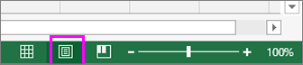
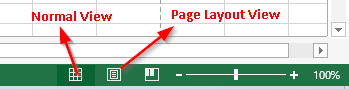
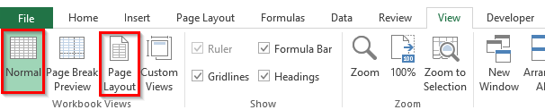
On the status bar, click the Page Layout View button.

-
Select the header or footer text you want to change.
-
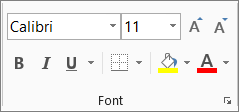
On the Home tab in the Font group, set the formatting options that you want to apply to the header / footer.
-
When you’re done, click the Normal view button on the status bar.
Prevent the header and footer font size from changing when you scale the worksheet for printing
If you don’t want the header and footer to scale with the document:
-
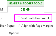
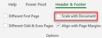
On the status bar, click the Page Layout View button, and then click Design and uncheck the Scale with Document box.
Tip: If you leave a check in the Scale with Document box, the header and footer font will scale along with the worksheet—and your header/footer Font settings likely won’t be reflected in the printout view.
For more information about working with titles, dates, and page numbers in headers and footers, see Headers and footers in a worksheet.
Need more help?
You can always ask an expert in the Excel Tech Community or get support in the Answers community.
Need more help?
Want more options?
Explore subscription benefits, browse training courses, learn how to secure your device, and more.
Communities help you ask and answer questions, give feedback, and hear from experts with rich knowledge.
See all How-To Articles
This tutorial demonstrates how to format headers and footers in Excel.
Format Header and Footer
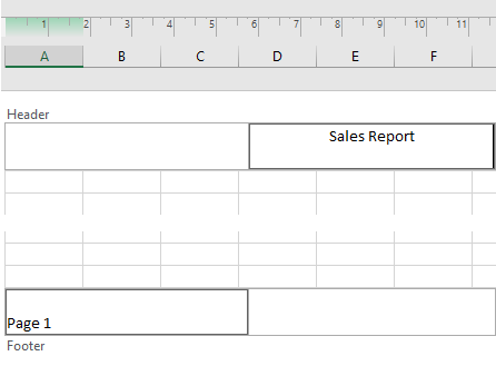
In Excel you can format the header and footer of your document, changing font style, size, color, etc. Say you already have the workbook with a header and footer, as in the picture below. (If you don’t already have a header or footer, see Insert Headers and Footers.)
To change the header format, follow these steps:
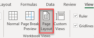
- To display the header and footer of your document, in the Ribbon, go to View > Page Layout.
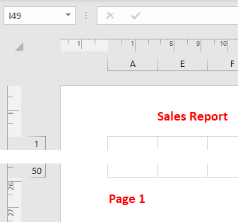
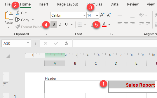
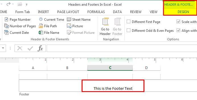
- Select the header (Sales Report), and in the Ribbon, go to Home. Set the font size (14), bold the text, and set font color (red).
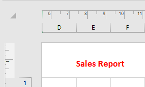
As a result, the header is formatted as you need it.
- Repeat Steps 1 and 2 to format the footer.
- To prevent the header and footer font from scaling along with the rest of the document, disable scaling with the document. Click the header or footer, and in the Ribbon, go to Header & Footer, and uncheck Scale with Document.
More on headers and footers…
- How to Insert Picture Into Header in Excel and Google Sheets
- How to Make a Header Only on the First Page in Excel
- How to Close Header and Footer in Excel and Google Sheets
- How to Add Element to Header to Display Current Date in Excel and Google Sheets
- How to View Header in Excel and Google Sheets
The header and footer are the document’s top and bottom portions, respectively. Similarly, Excel also has options for headers and footers. They are available in the “Insert” tab in the “Text” section. Using these features can provide us with two different spaces in the worksheet, one on the top and one on the bottom.
A header in excel: A worksheet section appears at the top of each Excel sheet or document page. It remains constant across all the pages. For example, it can contain page no., date, title, chapter name, etc.
Footer in Excel: A worksheet section appears at the bottom of each page in the Excel sheet or document. It remains constant across all the pages. It can contain page no., date, title, chapter name, etc.
The purpose of Header and Footer in Excel
The purpose is similar to that of hard copy documents or books. The headers and footers in Excel help meet the standard representation format of the documents and/or worksheets. In addition, they add a sense of organization to the soft documents and/or worksheets.
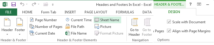
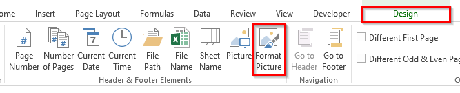
As we can see in the screenshot above, there are four sections under header and footer tools: “Header & Footer,” “Header & Footer Elements,” “Navigation,” and “Options.” This toolbox appears after clicking “Insert”-> “Header & Footer.”
- Header & Footer – This shows a list of the quick options as a header or footer.
- Header & Footer Elements – This has options for the text to be used as a header or footer, such as “Page Number,” “File Name,” “Number of Pages,” etc.
- Navigation – It has two options: “Go to Header” and “Go to Footer,” which navigates the cursor to the respective area.
- Options – It has two options related to putting up the header and footer conditionally: Different on the first page and Different on Odd & Even page. The other two options are regarding the formatting of the excelFormatting is a useful feature in Excel that allows you to change the appearance of the data in a worksheet. Formatting can be done in a variety of ways. For example, we can use the styles and format tab on the home tab to change the font of a cell or a table.read more page. One is to scale the header/footer with the document. The other is to align the header/footer with page margins.
Table of contents
- What are the Header and Footer in Excel?
- Header & Footer Tools in Excel
- How to Create a Header in Excel?
- How to Create Footer in Excel?
- How to Remove Header and Footer in Excel?
- How to Put Custom Text in Excel Header?
- How to Assign Page Number in Excel Footer Text?
- Things to Remember
- Recommended Articles
- Header & Footer Tools in Excel
Following are the steps for creating a header in Excel:
- First, click the worksheet where we want to add or change the header. Then, go to the “Insert tab” -“Text” group – “Header & Footer.”

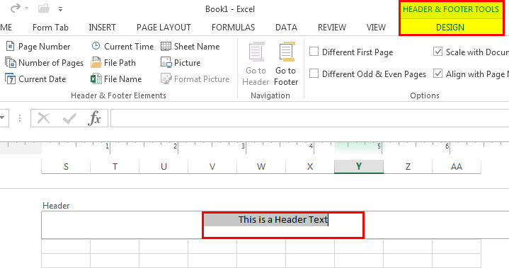
- Clicking on it would open a new window, as shown below.

- As shown in the screenshot below, “Header & Footer Tools” has a “Design” tab containing various text options to put as the header. The default is an empty text box wherein we can enter a free text, e.g., “This is the header text.” The other options are “Page Number,” “Number of Pages,” “Current Date,” “Current Time,” “File Path,” “File Name,” “Sheet Name,” “Picture,” etc.

- We must first click the worksheet where we want to add or change the header. Then, go to the “Insert” tab -> “Text” group -> “Header & Footer.”
- Clicking on it would open a new window, as shown. As shown in the screenshot below, “Header & Footer Tools” has a “Design” tab containing various text options to put as the header. The default is an empty text box wherein you can enter a free text, e.g., “This is the Footer text.” The other options are “Page Number,” “Number of Pages,” “Current Date,” “Current Time,” “File Path,” “File Name,” “Sheet Name,” “Picture,” etc.
How to Remove Header and Footer in Excel?
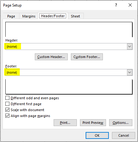
- We must first launch the “Page Setup” dialog box from the “Page Setup” box under the “Page Layout” menu.
- Then, go to the “Header/Footer” section.
- Select ‘none’ for “Header” and/or “Footer” to remove the respective feature.

How to Put Custom Text in Excel Header?
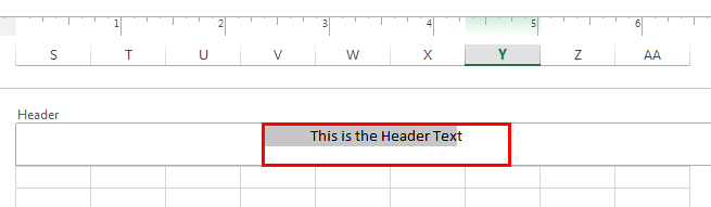
In the following example, “This is the Header Text” is the custom text entered in the “Header” box. The same will reflect on all the pages in the worksheet.
The “Header Text Editor” can be closed by pressing the “Escape” key on the keyboard.
How to Assign Page Number in Excel Footer Text?
The figure shows that a page number can be entered as the footer text. Refer to the screenshot below to understand the same.
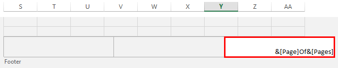
In the following example, “Page [&page] Of [&page]” is the text entered in the “Footer” box. Here, the “&[Page]Of” is a dynamic parameter that evaluates the page number. The first parameter is the current page number, and the second is the total number of pages. The same will reflect on all the pages in the worksheet.
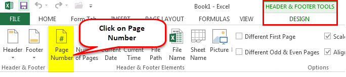
To give page numbers to a sheet, we must click on a sheet, go to “Footer,” click on the “Design” tab under “Header & Footer Tools,” and select “Page Number.”
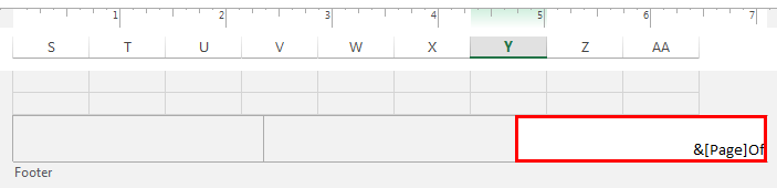
After “Selecting Page Numbers,” it will display as “&[Page]Of,” as shown in the below screenshot.
To show page numbers with total numbers of pages, we must click on the number of pages under the “Design” tab in the “Header & Footer” tool.
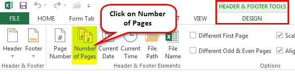
After selecting the number of pages, it will add “&[Page] Of &[Pages].
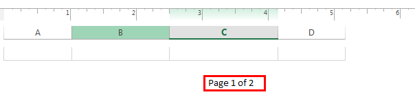
Then it shows the page number with the number of pages.
The “Footer Text Editor” can be closed by pressing the “Escape” key on the keyboard.
Note: In addition to the above-explained examples, the other options for header/footer text made available by MS Excel are “Date,” “Time,” “File Name,” “Sheet Name,” etc.
Things to Remember
- The headers and footers in Excel help meet the standard representation format of the documents or worksheets.
- They add a sense of organization to the soft documents.
- Excel offers various options to be put up as header/footer text, such as “Date,” “Time,” “Sheet Name,” “File Name,” “Page Number,” “Custom Text,” etc.
Recommended Articles
This article is a guide to Header and Footer in Excel. Here, we discuss creating and removing the header and footer in Excel,, practical examples,, and a downloadable Excel template. You may learn more about Excel from the following articles: –
- VBA Text Box
- Formula to Add Text in Excel
- Circular Reference in Excel
- Insert Row Excel Shortcut
- PI in Excel
Excel Header Row (Table of Contents)
- Header Row in Excel
- How to turn the Row Header on or off in Excel?
- Row Header formatting options in Excel
Microsoft Excel sheet has the capacity to hold a million rows with a numeric or text dataset in it.
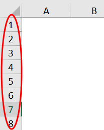
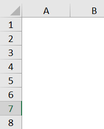
Row header or Row heading is the gray-colored column located on the left side of column 1 in the worksheet, which contains the numbers (1, 2, 3, etc.) where it helps out to identify each row in the worksheet. Whereas the column header is the gray-colored row, it will usually be letters (A, B, C, etc.), which helps identify each column in the worksheet.
Row header label will help you out to identify & compare the information of the content when you are working with a huge number of data sets when it is difficult to accommodate the data in a single window or page & to compare information in your worksheet of excel.
Usually, a combination of column letters and row numbers helps out to create cell references. Row header will help you identify individual cells located at the intersection point between a column and row in a worksheet in excel.
Definition
Header rows are the label rows containing information that helps you identify the content of a particular column in a worksheet.
If the dataset table spans over several pages in an excel sheet print layout or towards the right if you scroll on & on, the header row will remain constant & stagnant, which usually repeat itself at the beginning of each new page.
How to turn the Header Row on or off in Excel?
Row headers in excel will always be visible all the time, even when you scroll the column data sets or values towards the right in the worksheet.
Sometimes, the row header in excel will not be displayed on a particular worksheet. It will be turned off in several cases, the main reason for turning them off is –
- Better or improved appearance of the worksheet in excel or
- To obtain or gain the extra screen space on worksheets containing a large number of tabular datasets.
- To take a screenshot or capture.
- When you take a printout of a tabular dataset, the row header or heading makes things complicated or confusing with the printed data set because of interference of row & column header; therefore, whenever you take a print out, the row header should always be turned off for each individual worksheet in the excel.
Now, let’s check out how to turn off the row headers or headings in Excel.
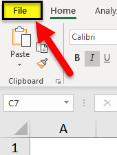
- Select or Click on the File option in the home toolbar of the menu to open the drop-down list.
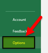
- Click on Options in the list present on the left-hand side to open the Excel Options dialog box.
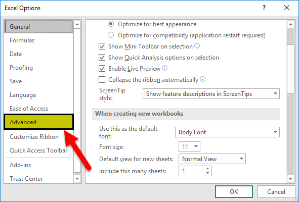
- Now, the Excel Options dialog box appears; in the left-hand panel of the excel options dialog box, select the Advanced option.
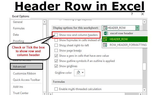
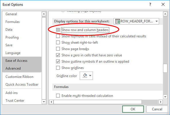
- Now, if you move the cursor down after the advanced option, you can observe Display options for this worksheet section located near the bottom of the right-hand pane of the dialog box; by default, it shows the row and column headers option always checked or ticked in.
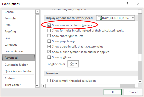
- If you want to turn off the row headers or headings in Excel, click on or uncheck the selection box of a checkbox in the Show row and column headers option.
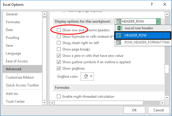
- Simultaneously, you can turn off the row and column headings for additional worksheets in the open workbook or current workbook of excel. It can be done by selecting the name of another worksheet under the drop-down box located next to the Display options.
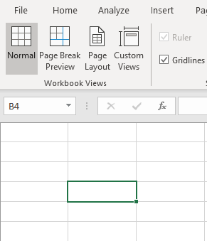
- Once you have unchecked the box, Click OK to close the excel options dialog box, and you can return to the worksheet.
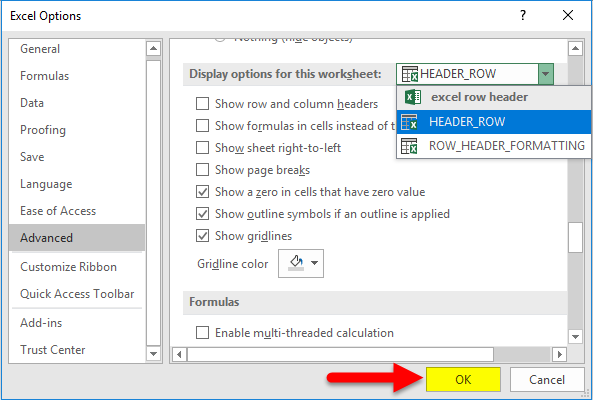
- Now, the above procedure disables the visibility of a row or column header.
When you try to open a new Excel file, the row header or heading is displayed by default of normal style or theme font similar to the workbook’s default format. This same normal style font is also applicable for all the worksheet in the workbook.
The default heading font is Calibri & the font size is 11. It can be changed based on your choice as per your requirement; whatever font style & size you apply will reflect in all the worksheets in a workbook of excel.
You have an option to format font & its size settings, with various options in format settings.
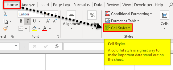
- In the Home tab of the Ribbon menu. Under the Styles group, select or click on Cell Styles to open the Cell Styles drop-down palette.
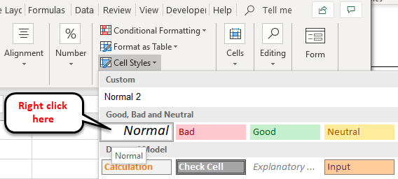
- In the dropdown, under Good, bad & neutral, Right-click or select on the box in the palette entitled Normal – it is also called a Normal style.
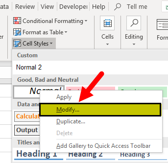
- Click on Modify option under normal.
- A style dialog box appears; click on the Format in that window.
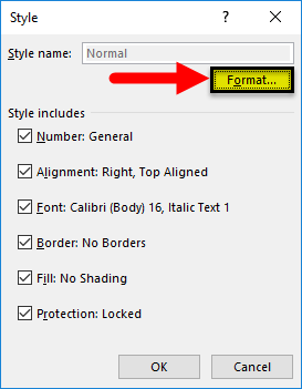
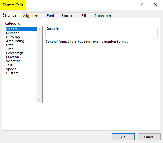
- Now, the Format Cells dialog box appears. In that, you can change the font size and its appearance, i.e. Font style or size.
- I changed the font style & size, i.e. Calibri & font style to Regular, and I increased the font size to 16 from 11.
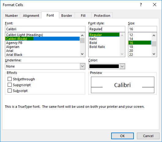
Once the desired changes are made, click OK twice, i.e. in the format cells dialog box & style dialog box based on your preference.
Note: Once you made changes in the font settings, you have to click on the save option in the workbook; otherwise, it will revert back to the default normal style or theme font (i.e.default heading font is Calibri & font size is 11).
Things to Remember
- Row header (with row number) make things easier to view or access the content when you try to navigate or scroll to another area or different parts of your worksheet at the same time in excel.
- An advantage of the header row is you can set this label row to print on all pages in excel or word; it is very significant & will be helpful for spreadsheets that span multiple pages.
Recommended Articles
This has been a guide to Header Row in Excel. Here we discuss how to turn row header on or off and row header formatting options in excel. You can also go through our other suggested articles –
- ROWS Function in Excel
- Column Header in Excel
- Excel Header and Footer
- Add Rows in Excel Shortcut
Содержание
- Создание наименования
- Этап 1: создание места для названия
- Этап 2: внесение наименования
- Этап 3: форматирование
- Этап 4: закрепление названия
- Этап 5: печать заголовка на каждой странице
- Вопросы и ответы

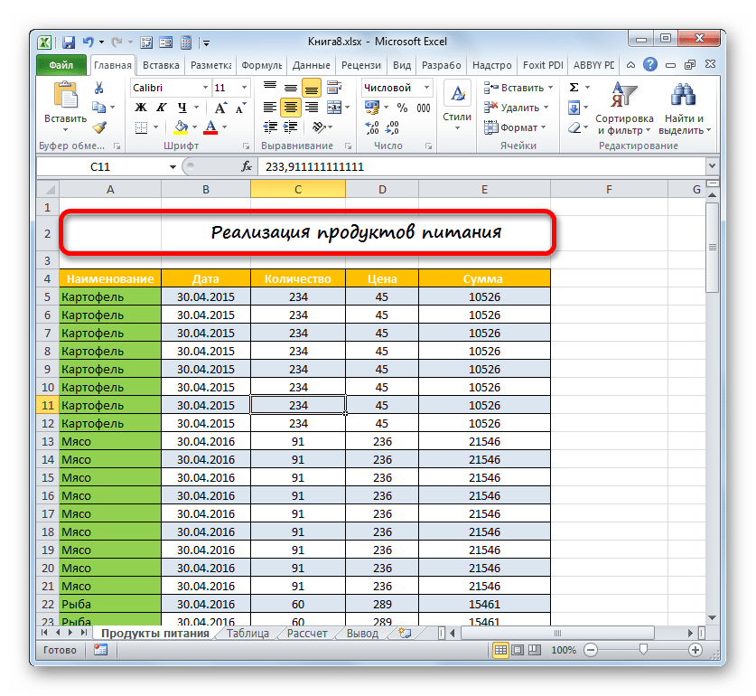
Визитной карточкой любого документа является его название. Этот постулат также относится и к таблицам. Действительно, намного приятнее видеть информацию, которая отмечена информативным и красиво оформленным заголовком. Давайте узнаем алгоритм действий, которые следует выполнить, чтобы при работе с таблицами Excel у вас всегда были качественные наименования таблиц.
Создание наименования
Основным фактором, при котором заголовок будет выполнять свою непосредственную функцию максимально эффективно, является его смысловая составляющая. Наименование должно нести основную суть содержимого табличного массива, максимально точно описывать его, но при этом быть по возможности короче, чтобы пользователь при одном взгляде на него понял, о чем речь.
Но в данном уроке мы все-таки больше остановимся не на таких творческих моментах, а уделим основное внимание алгоритму технологии составления наименования таблицы.
Этап 1: создание места для названия
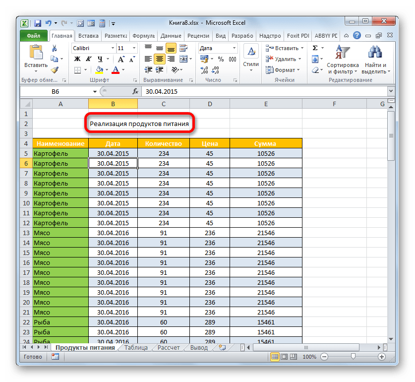
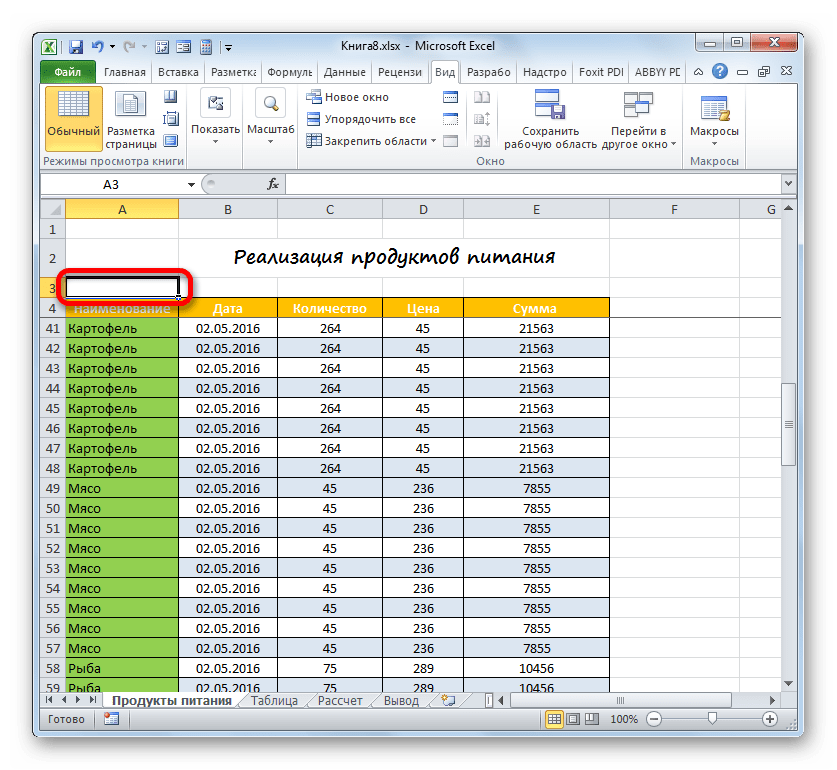
Если вы уже имеете готовую таблицу, но вам нужно её озаглавить, то, прежде всего, требуется создать место на листе, выделенное под заголовок.
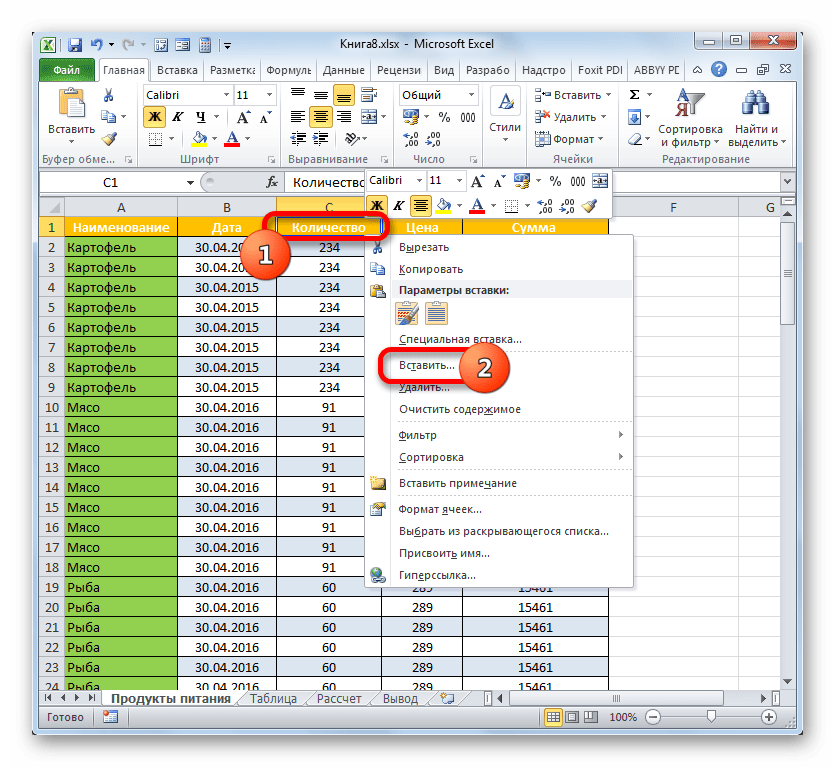
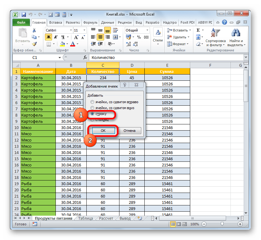
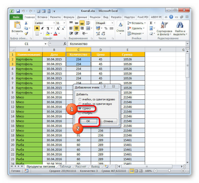
- Если табличный массив своей верхней границей занимает первую строчку листа, то требуется расчистить место для названия. Для этого устанавливаем курсор в любой элемент первой строчки таблицы и клацаем по нему правой кнопкой мыши. В открывшемся меню выбираем вариант «Вставить…».
- Перед нами предстает небольшое окно, в котором следует выбрать, что конкретно требуется добавить: столбец, строку или отдельные ячейки с соответствующим сдвигом. Так как у нас поставлена задача добавления строки, то переставляем переключать в соответствующую позицию. Клацаем по «OK».
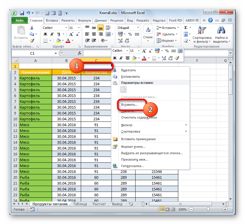
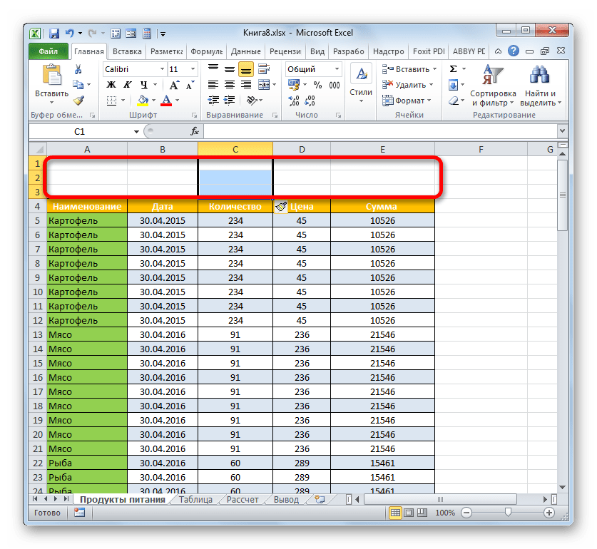
- Над табличным массивом добавляется строка. Но, если добавить между наименованием и таблицей всего одну строчку, то между ними не будет свободного места, что приведет к тому, что заголовок не будет так выделяться, как хотелось бы. Это положение вещей устраивает не всех пользователей, а поэтому есть смысл добавить ещё одну или две строки. Для этого выделяем любой элемент на пустой строке, которую мы только что добавили, и клацаем правой кнопкой мыши. В контекстном меню снова выбираем пункт «Вставить…».
- Дальнейшие действия в окошке добавления ячеек повторяем точно так же, как было описано выше. При необходимости таким же путем можно добавить ещё одну строчку.
Но если вы хотите добавить больше одной строчки над табличным массивом, то существует вариант значительно ускорить процесс и не добавлять по одному элементу, а сделать добавление одним разом.
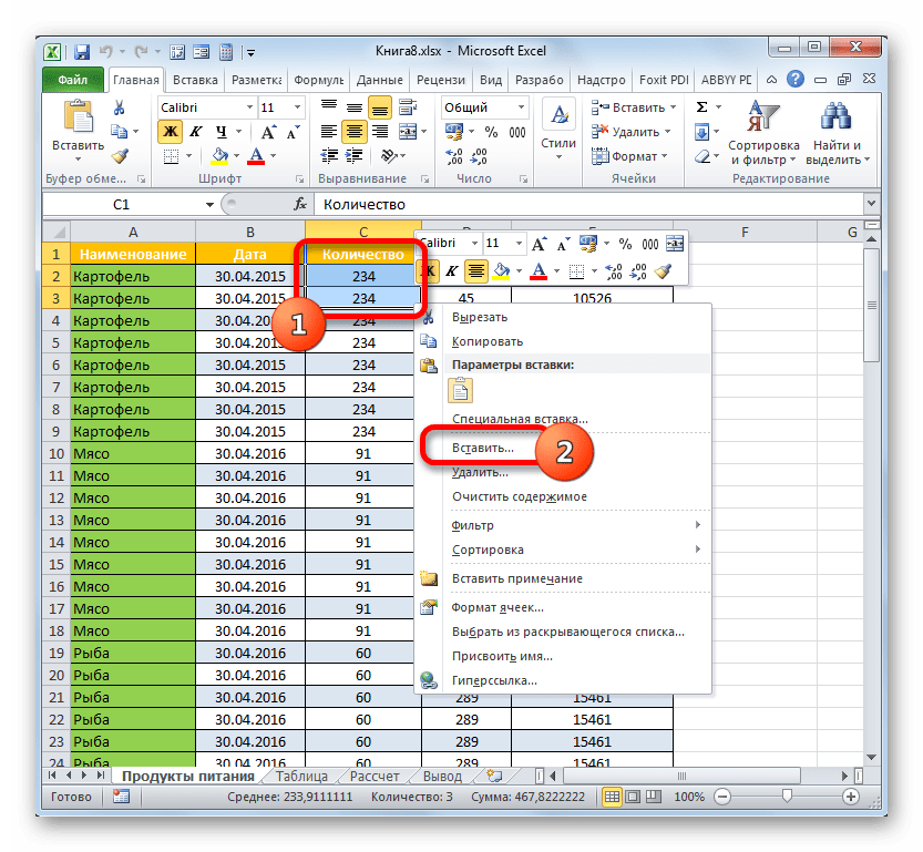
- Выделяем вертикальный диапазон ячеек в самом верху таблицы. Если вы планируете добавить две строчки, то следует выделить две ячейки, если три – то три и т.д. Выполняем клик по выделению, как это было проделано ранее. В меню выбираем «Вставить…».
- Опять открывается окошко, в котором нужно выбрать позицию «Строку» и нажать на «OK».
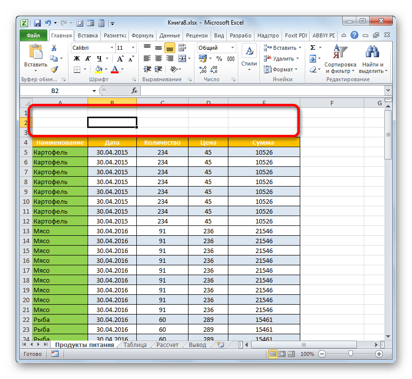
- Над табличным массивом будет добавлено то количество строк, сколько элементов было выделено. В нашем случае три.
Но существует ещё один вариант добавления строк над таблицей для наименования.
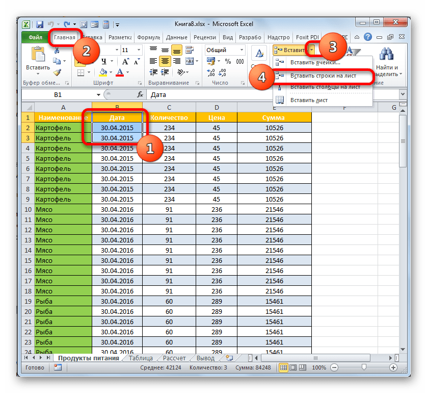
- Выделяем вверху табличного массива столько элементов в вертикальном диапазоне, сколько строк собираемся добавить. То есть, делаем, как в предыдущих случаях. Но на этот раз переходим во вкладку «Главная» на ленте и щелкаем по пиктограмме в виде треугольника справа от кнопки «Вставить» в группе «Ячейки». В списке выбираем вариант «Вставить строки на лист».
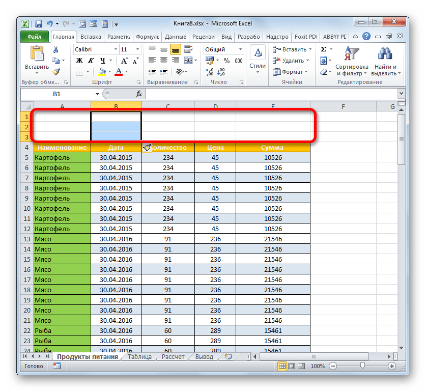
- Происходит вставка на лист выше табличного массива того количества строк, сколько ячеек перед тем было отмечено.

На этом этап подготовки можно считать завершенным.
Урок: Как добавить новую строку в Экселе
Этап 2: внесение наименования
Теперь нам нужно непосредственно записать наименование таблицы. Каким должен быть по смыслу заголовок, мы уже вкратце говорили выше, поэтому дополнительно на этом вопросе останавливаться не будем, а уделим внимание только техническим моментам.
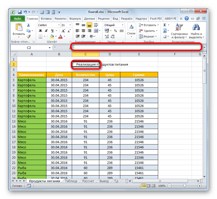
- В любой элемент листа, расположенный над табличным массивом в строках, которые мы создали на предыдущем этапе, вписываем желаемое название. Если над таблицей две строки, то лучше это сделать в самой первой из них, если три – то в расположенной посередине.
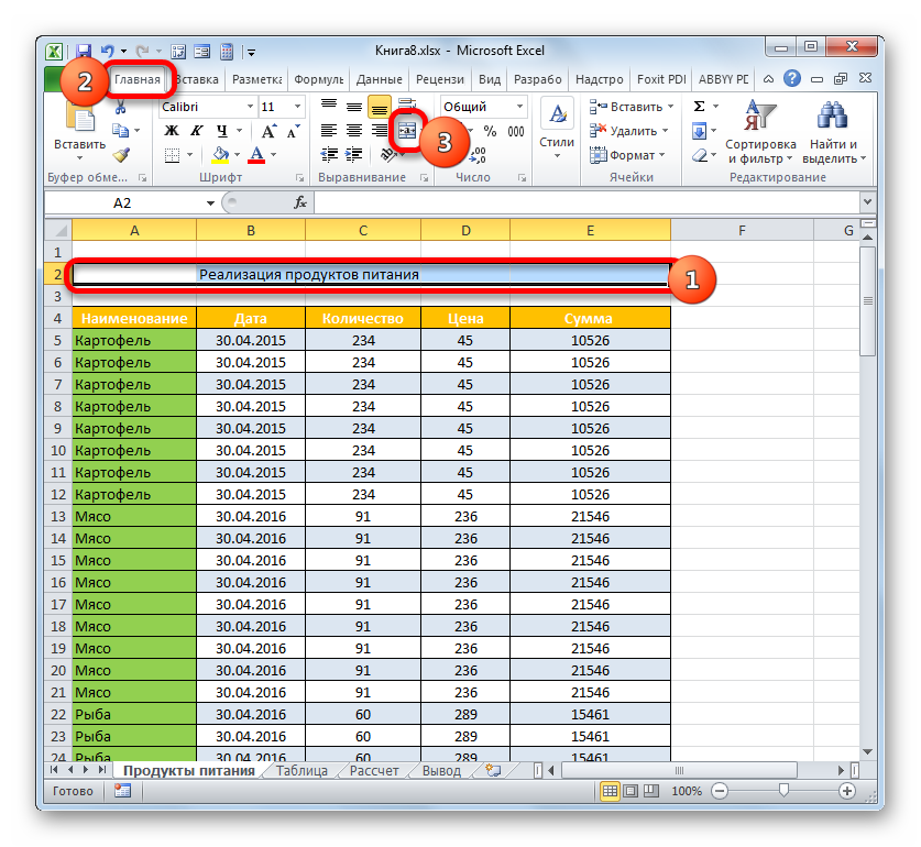
- Теперь нам нужно расположить данное наименование посередине табличного массива для того, чтобы оно выглядело более презентабельно.
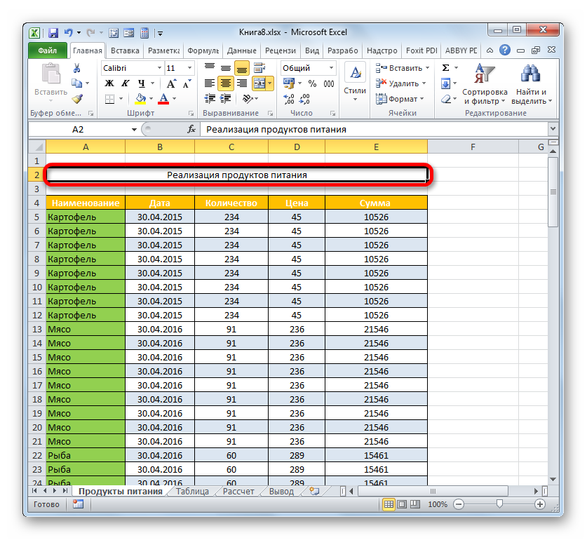
Выделяем весь диапазон ячеек, находящийся над табличным массивом в той строчке, где размещено наименование. При этом левая и правая границы выделения не должны выходить за соответствующие границы таблицы. После этого жмем на кнопку «Объединить и поместить в центре», которая имеет место расположения во вкладке «Главная» в блоке «Выравнивание».
- После этого элементы той строчки, в которой расположено наименование таблицы, будут объединены, а сам заголовок помещен в центре.
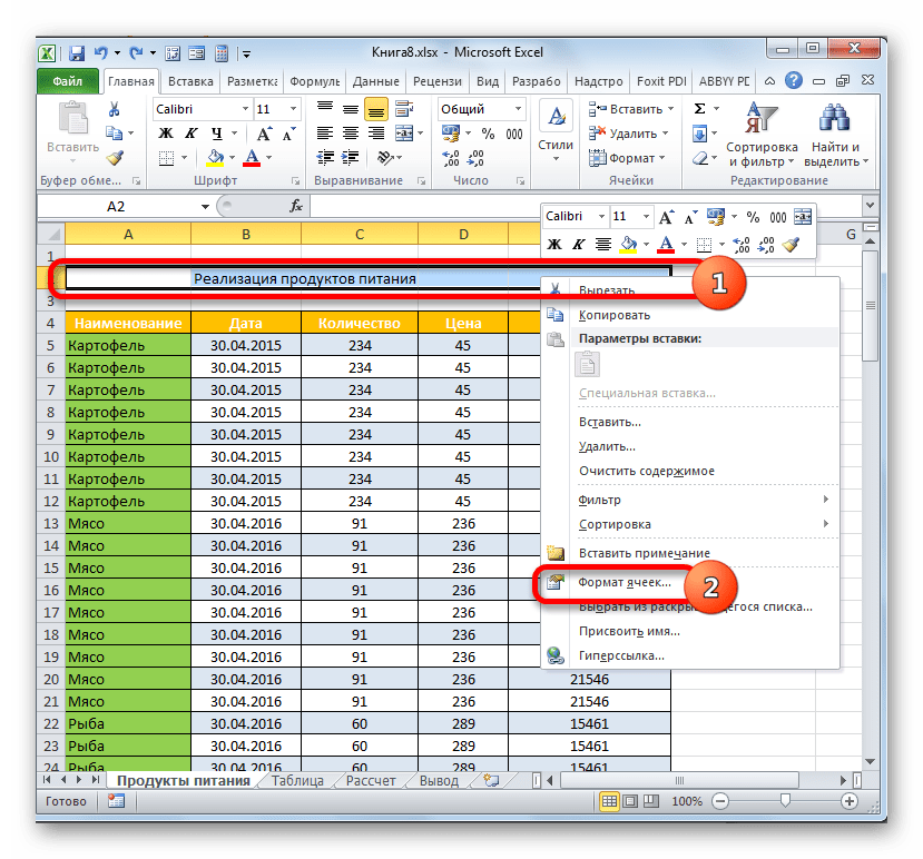
Существует ещё один вариант объединения ячеек в строке с наименованием. Его реализация займет немногим больший отрезок времени, но, тем не менее, данный способ тоже следует упомянуть.
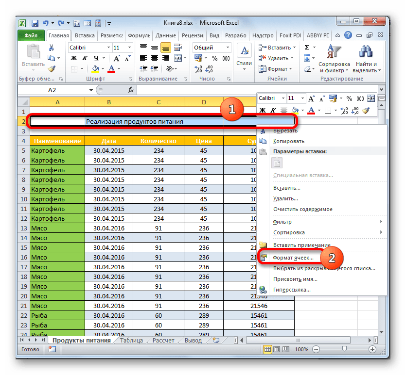
- Производим выделение элементов листа строчки, в которой расположено наименование документа. Клацаем по отмеченному фрагменту правой кнопкой мыши. Выбираем в списке значение «Формат ячеек…».
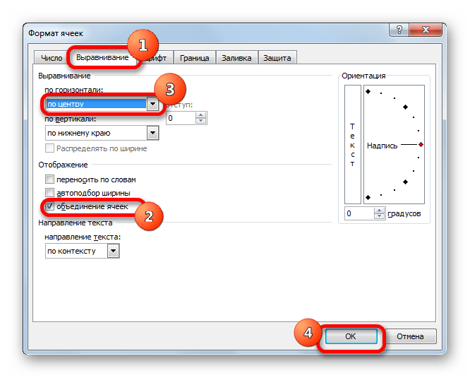
- В окне форматирования производим перемещение в раздел «Выравнивание». В блоке «Отображение» выполняем установку флажка около значения «Объединение ячеек». В блоке «Выравнивание» в поле «По горизонтали» устанавливаем значение «По центру» из списка действий. Щелкаем по «OK».
- В этом случае ячейки выделенного фрагмента также будут объединены, а наименование документа помещено в центр объединенного элемента.

Но в некоторых случаях объединение ячеек в Экселе не приветствуется. Например, при использовании «умных» таблиц к нему лучше вообще не прибегать. Да и в других случаях любое объединение нарушает изначальную структуру листа. Что же делать, если пользователь не хочет объединять ячейки, но вместе с тем желает, чтобы название презентабельно размещалось по центру таблицы? В этом случае также существует выход.
- Выделяем диапазон строчки над таблицей, содержащей заголовок, как мы это делали ранее. Клацаем по выделению для вызова контекстного меню, в котором выбираем значение «Формат ячеек…».
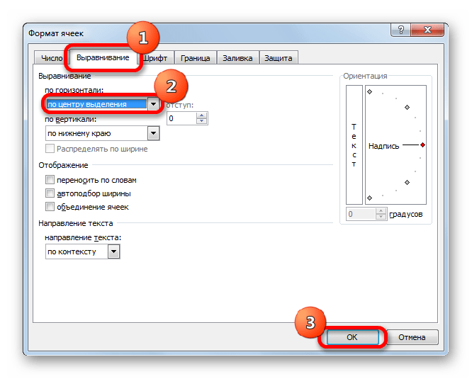
- В окне форматирования перемещаемся в раздел «Выравнивание». В новом окне в поле «По горизонтали» выбираем в перечне значение «По центру выделения». Клацаем по «OK».
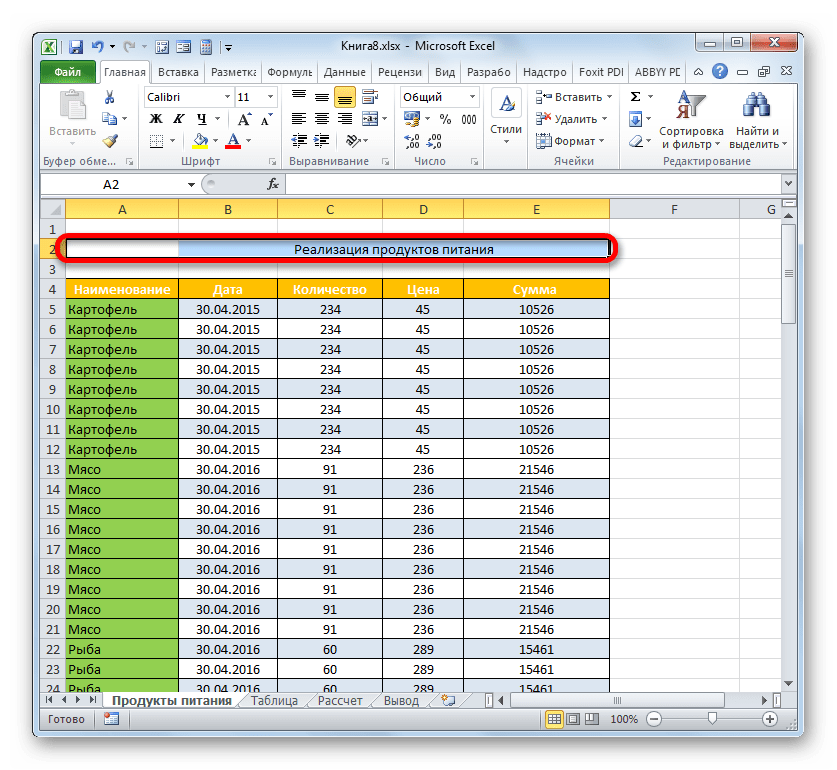
- Теперь наименование будет отображаться по центру табличного массива, но при этом ячейки не будут объединены. Хотя будет казаться, что название размещено посередине, физически его адрес соответствует тому изначальному адресу ячейки, в которой оно было записано ещё до процедуры выравнивания.
Этап 3: форматирование
Теперь настало время отформатировать заголовок, чтобы он сразу бросался в глаза и выглядел максимально презентабельным. Сделать это проще всего при помощи инструментов форматирования на ленте.
- Отмечаем заголовок кликом по нему мышки. Клик должен быть сделан именно по той ячейке, где физически название находится, если было применено выравнивание по выделению. Например, если вы кликните по тому месту на листе, в котором отображается название, но не увидите его в строке формул, то это значит, что фактически оно находится не в данном элементе листа.

Может быть обратная ситуация, когда пользователь выделяет с виду пустую ячейку, но в строке формул видит отображаемый текст. Это означает, что было применено выравнивание по выделению и фактически название находится именно в этой ячейке, несмотря на то, что визуально это выглядит не так. Для процедуры форматирования следует выделять именно данный элемент.
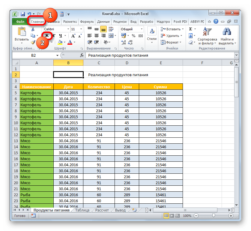
- Выделим наименование полужирным шрифтом. Для этого кликаем по кнопке «Полужирный» (пиктограмма в виде буквы «Ж») в блоке «Шрифт» во вкладке «Главная». Или применяем нажатие комбинации клавиш Ctrl+B.
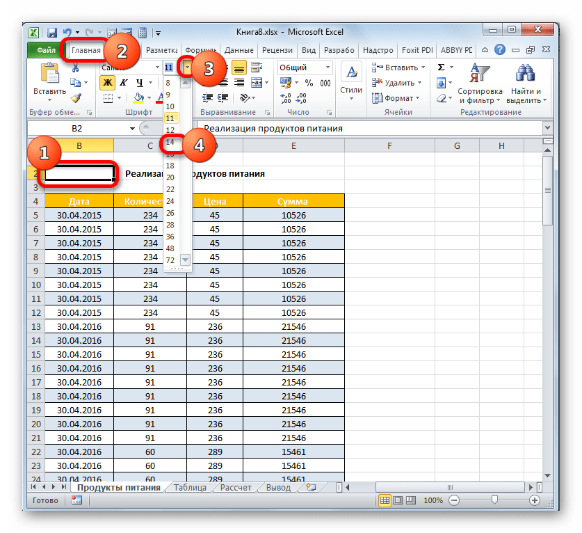
- Далее можно увеличить размер шрифта названия относительно другого текста в таблице. Для этого опять выделяем ячейку, где фактически расположено наименование. Кликаем по пиктограмме в виде треугольника, которая размещена справа от поля «Размер шрифта». Открывается список размеров шрифта. Выбирайте ту величину, которую вы сами посчитаете оптимальной для конкретной таблицы.
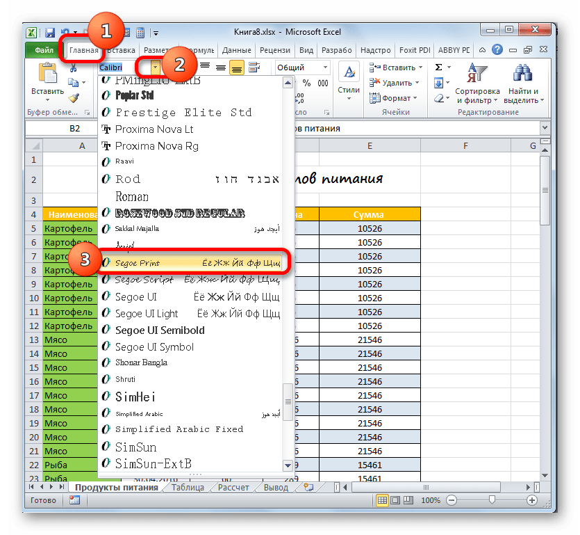
- Если есть желание, можно также изменить наименование типа шрифта на какой-нибудь оригинальный вариант. Клацаем по месту размещения наименования. Кликаем по треугольнику справа от поля «Шрифт» в одноименном блоке во вкладке «Главная». Открывается обширный перечень типов шрифтов. Щелкаем по тому, который вы считаете более уместным.
Но при выборе типа шрифта нужно проявлять осторожность. Некоторые могут быть просто неуместными для документов определенного содержания.

При желании форматировать наименование можно практически до бесконечности: делать его курсивом, изменять цвет, применять подчеркивание и т. д. Мы же остановились только на наиболее часто используемых элементах форматирования заголовков при работе в Экселе.
Урок: Форматирование таблиц в Майкрософт Эксель
Этап 4: закрепление названия
В некоторых случаях требуется, чтобы заголовок был постоянно на виду, даже если вы прокручиваете длинную таблицу вниз. Это можно сделать путем закрепления строки наименования.
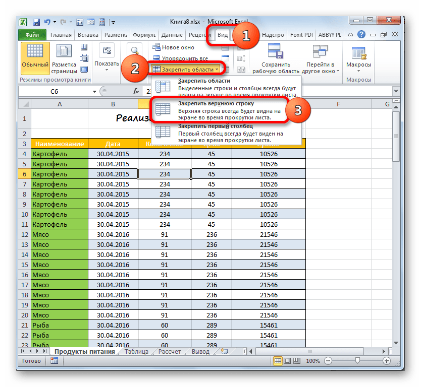
- Если название находится в верхней строчке листа, сделать закрепление очень просто. Перемещаемся во вкладку «Вид». Совершаем клик по иконке «Закрепить области». В списке, который откроется, останавливаемся на пункте «Закрепить верхнюю строку».
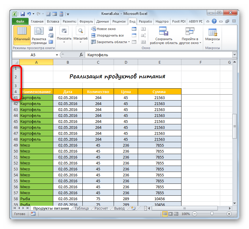
- Теперь верхняя строчка листа, в которой находится название, будет закреплена. Это означает, что она будет видна, даже если вы опуститесь в самый низ таблицы.

Но далеко не всегда название размещается именно в верхней строчке листа. Например, выше мы рассматривали пример, когда оно было расположено во второй строчке. Кроме того, довольно удобно, если закреплено не только наименование, но и шапка таблицы. Это позволяет пользователю сразу ориентироваться, что означают данные, размещенные в столбцах. Чтобы осуществить данный вид закрепления, следует действовать по несколько иному алгоритму.
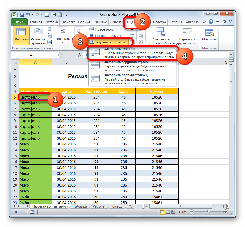
- Выделяем крайнюю левую ячейку под той областью, которая должна быть закреплена. В данном случае мы закрепим сразу заголовок и шапку таблицы. Поэтому выделяем первую ячейку под шапкой. После этого жмем по иконке «Закрепить области». На этот раз в списке выбираем позицию, которая так и называется «Закрепить области».
- Теперь строки с названием табличного массива и его шапка будут закреплены на листе.
Если же вы все-таки желаете закрепить исключительно название без шапки, то в этом случае нужно перед переходом к инструменту закрепления выделить первую левую ячейку, размещенную под строчкой названия.
Все остальные действия следует провести по точно такому же алгоритму, который был озвучен выше.
Урок: Как закрепить заголовок в Экселе
Этап 5: печать заголовка на каждой странице
Довольно часто требуется, чтобы заголовок распечатываемого документа выходил на каждом его листе. В Excel данную задачу реализовать довольно просто. При этом название документа придется ввести только один раз, а не нужно будет вводить для каждой страницы отдельно. Инструмент, который помогает воплотить данную возможность в реальность, имеет название «Сквозные строки». Для того, чтобы полностью завершить оформление названия таблицы, рассмотрим, как можно осуществить его печать на каждой странице.
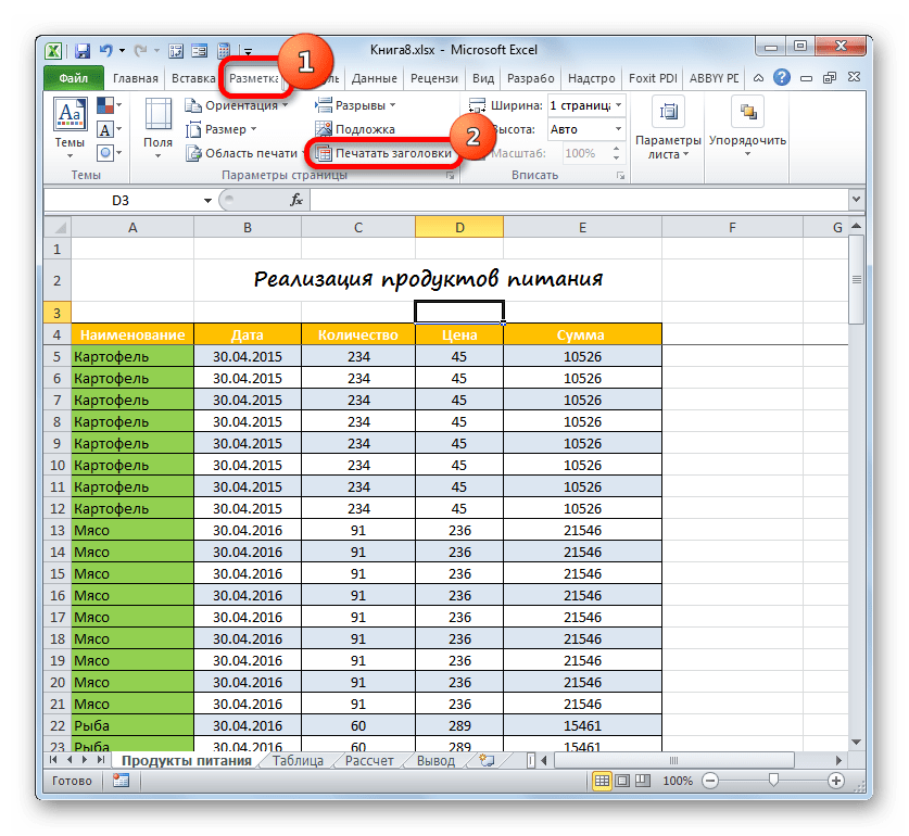
- Совершаем передвижение во вкладку «Разметка». Клацаем по значку «Печатать заголовки», который расположен в группе «Параметры страницы».
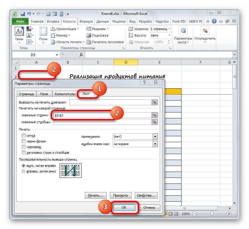
- Активируется окно параметров страницы в разделе «Лист». Ставим курсор в поле «Сквозные строки». После этого выделяем любую ячейку, находящуюся в строчке, в которой размещен заголовок. При этом адрес всей данной строки попадает в поле окна параметров страницы. Кликаем по «OK».
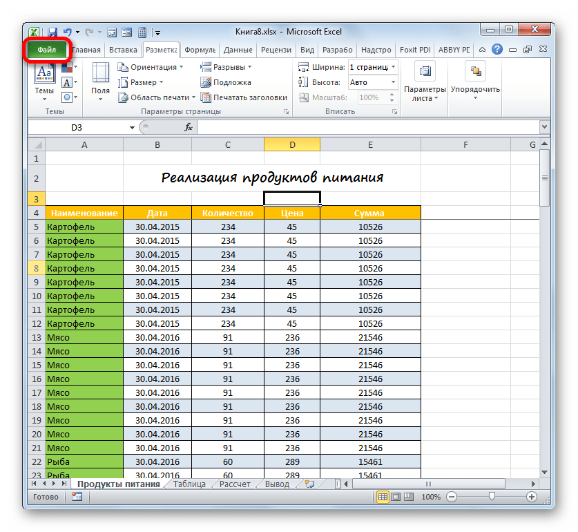
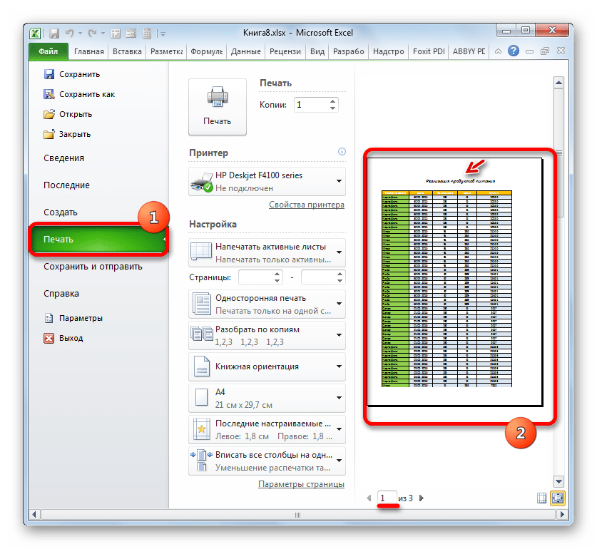
- Для того, чтобы проверить, как будут отображаться заголовок при печати, переходим во вкладку «Файл».
- Перемещаемся в раздел «Печать» с помощью инструментов навигации левого вертикального меню. В правой части окна размещена область предварительного просмотра текущего документа. Ожидаемо на первой странице мы видим отображаемый заголовок.
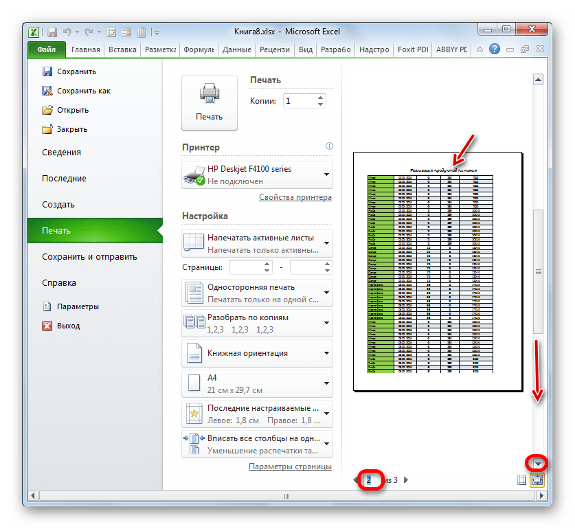
- Теперь нам нужно взглянуть на то, будет ли отображаться название на других печатных листах. Для этих целей опускаем полосу прокрутки вниз. Также можно ввести номер желаемой страницы в поле отображения листов и нажать на клавишу Enter. Как видим, на втором и последующих печатных листах заголовок также отображается в самом вверху соответствующего элемента. Это означает то, что если мы пустим документ на распечатку, то на каждой его странице будет отображаться наименование.
На этом работу по формированию заголовка документа можно считать завершенной.
Урок: Печать заголовка на каждой странице в Экселе
Итак, мы проследили алгоритм оформления заголовка документа в программе Excel. Конечно, данный алгоритм не является четкой инструкцией, от которой нельзя отходить ни на шаг. Наоборот, существует огромное количество вариантов действий. Особенно много способов форматирования названия. Можно применять различные сочетания многочисленных форматов. В этом направлении деятельности ограничителем является только фантазия самого пользователя. Тем не менее, мы указали основные этапы составления заголовка. Данный урок, обозначив основные правила действий, указывает на направления, в которых пользователь может осуществлять собственные задумки оформления.
Do you know that excel also provides with the Header and Footer Feature in Excel? In this blog, we would learn how to insert or make a header in Excel. We would also go through some of the pre-defined excel header and footer and also learn how to create our own custom header or footer in Excel.
Excel Headers and Footers are the text or images placed on the top and bottom of each of the pages respectively. These texts/images provide some basic information about the pages or the document like the title of the document, page number, company logo, date/time, etc.
Table of Contents
- Brief Information on Excel Headers and Footers
- Navigating to Header and Footer Feature in Excel
- How to Insert Excel Preset Header and Footer
- Using Page Setup Dialog Box
- Using Insert Header and Footer – Design Tab
- Custom Header and Footer Using Elements
- Using Combination of Elements to Customize Headers and Footers
- Insert Picture or Image in Excel Header or Footer
- Add Headers and Footers in Multiple Sheets at One Go
- Other Miscellaneous Options In Design Tab
- How to Change Font Size and Color of Header and Footer in Excel
- Show or Hide Header and Footer in Excel
- Remove or Delete Header and Footer in Excel
Microsoft has given many standard headers and footers which are inbuilt to excel. Additionally, you can also create your own customized ones to make a more good looking excel document and reports.
In excel, the headers and footer feature is available at two places.
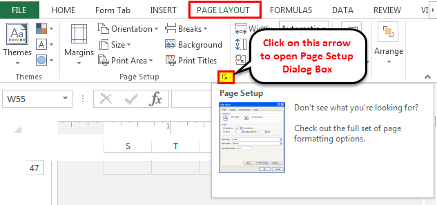
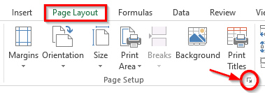
- Go to the ribbon tab Page Layout. Under the Page Setup group, you would find a small icon on the bottom right corner. This is the dialog box launcher. Click on it and the Page Setup dialog box would appear on the screen. There, you can find a specific tab named – Header/Footer.
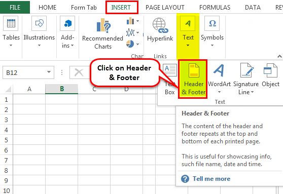
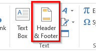
- Additionally, you would find the Excel headers and footers feature under the ‘Insert‘ Tab. Click on the ‘Insert‘ tab > ‘Text‘ group > Header & Footer Option.
Now, when you know the path for navigating to this feature, let us begin with exploring this rarely used feature.
As mentioned in the introduction of this blog, excel has provided with some pre-defined headers and footers that you can use. To insert the preset headers and footer, you can use either of the navigation paths. Let us check on both of these.
Using Page Setup Dialog Box
- Navigate to the Page Setup dialog box > Header/Footer tab (as learned in previous section).
- The option ‘None‘ (shown in the screenshot below) means at present no headers/footers are put in the worksheet.
- Click on the ‘Header‘ drop-down option arrow and there you would find many available header options provided by Microsoft. Select one of your choices. Similarly, under the ‘Footer‘ drop-down option, you can find and select the one from the available default footers.
For example, I have chosen to insert the workbook or file name as headers and the current sheet’s name and the page number as the footer part. See the image below:
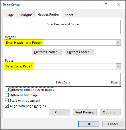
As soon as you press the OK button, the dialog box would exit, and excel would insert the headers and footer on the active worksheet.
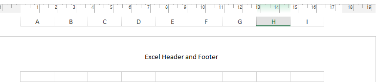
Header looks like this:
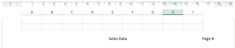
Footer looks like this:
Using Insert Header and Footer – Design Tab
- Go to the Insert tab and click on the option – Header & Footer (under Text group).
- This would instantly and quickly create a structure of excel headers and footers in the worksheet. Simultaneously, excel also inserts a new tab in the ribbon with the name ‘Design‘ (as shown below).
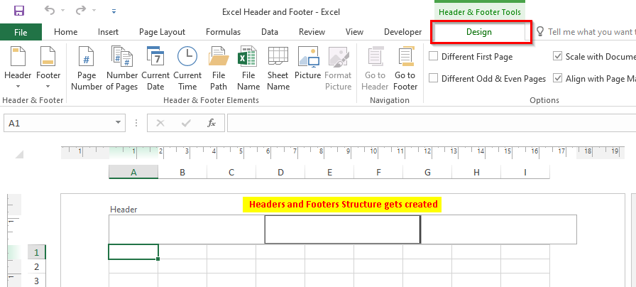
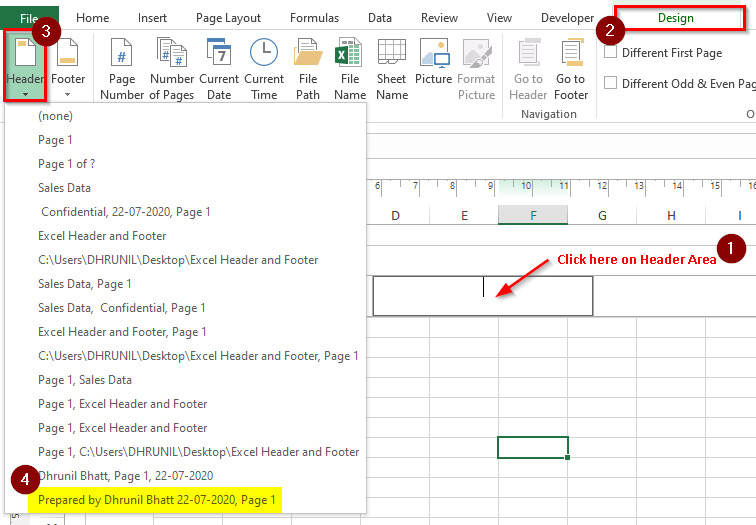
- To insert preset excel headers, click on the header structure in the worksheet area. Under the Design tab, click on the option that says ‘Header‘. As a result, a drop-down list of all the available predefined excel headers would be displayed. Select one of your choices and that’s it.
- Similarly, to insert footer from the predefined list of footers, click on the option that says ‘Footer‘ under the ‘Design’ Tab > ‘Header & Footer’ group. From the list of drop-down options, select one of your choices, and you are done.
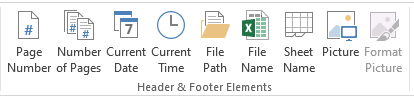
In addition to the predefined headers and footers, you can also create custom ones by using the Header and Footer Elements. These elements are available in the ‘Design‘ tab, as shown in the image below:
Procedure to use and insert these elements:
- Click on the appropriate header area. Let us first enter the middle part of the header.
- Now, go to the ‘Design‘ tab in the ribbon and select the element to insert, for example, FileName. Click on the option – File Name, and as a result, excel would insert the word &[File] there.
- To see the exact header text, click anywhere on the worksheet.
In a similar manner, you can insert the left and right parts of the header by selecting the part and then following the above procedure.
When you are on the header part and you want to move to the footer part, there are two possible ways to do so:
- The first one is to use the right scroll bar to move downwards until you see the footer.
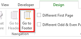
- The second and the most prominent one is to use the option – ‘Go To Footer‘ (Design Tab). By clicking on this, you would instantly jump to the Footer part.
Using Combination of Elements to Customize Headers and Footers
One interesting thing with using the custom header or footer in excel is that you can use a combination of multiple elements. Suppose, we want to show the page number in the footer in this format – Page <Current Page No.> of <Total Pages> (For Eg – Page 1 of 19). There is no element to achieve this.
However, you can use the combination of two elements – Page Number and Number of Pages to get the required text. The below demonstration is self-explanatory.

Follow Below Steps to Insert Image or Picture in Header and Footer in Excel
- Navigation
Click on the appropriate header or footer area and go to the ‘Design‘ Tab.
- Picture Element
Under the ‘Header and Footer Elements’ click on the element that says – ‘Picture‘.
- Insert Picture Dialog Box
In the ‘Insert Picture’ dialog box that appears, search for the picture that you want to insert and click on the ‘Insert’ button.
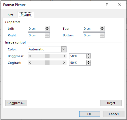
As a result, the excel would insert the picture inside the header or footer. Once the picture is inserted in the header or footer, the ‘Format Picture‘ element gets activated.
You can resize the picture inside the header or footer, increase picture height or width. You can also, set the top, left, bottom, and right alignment of the picture using this option. Excel also provides you with the option to change the color setting (including brightness and contrast).
When you insert a header or a footer using the method(s) stated above, it only gets added to the active sheet. Header and Footer do not apply to all the worksheets in the excel workbook.
To do so, you need to first group the worksheets and then perform the above steps to add header or footer to all those grouped worksheets.
Make sure that you remember to ungroup the grouped worksheets once your task is over.
I have an exclusive blog on Grouping and Ungrouping Worksheets in Excel. To read it, click here.
Other Miscellaneous Options In Design Tab
There are four miscellaneous but very important checkboxes in the Header and Footer Design Tab which are explained below:
- Different First Page – When you want to have a different header or footer for the first page, tick this checkbox and then give a separate header and footer for the first page. For the other pages, you need to again give a header or footer only on the second page and it would be applicable for all the pages (except for the first page).
- Different Odd & Even Pages – As the name suggests, tick this checkbox, if you want that the odd pages (1, 3, 5, and so on) should have different headers/footers than the even pages (2, 4, 6, and so on).
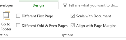
- Scale with Document – The scale with document checkbox is ticked by default. A tick means when you change the scale of the document (while printing), the header and footer font size will also change accordingly. To stop changing the header and footer size while scaling the document for printing, uncheck this option.
- Align with Page Margin – It is better to have this option activated so that the headers and footers are aligned according to the page margin.
To change the font settings of the header and footer, simply select the header or footer using the mouse (keyboard shortcut selection would not work).
A small font formatting dialog box would appear on your screen. Use the font formatting options as per your need, as shown in the below demonstration.
You can show or hide the header and footer in Excel by toggling between Normal view and the Page Layout view. See the below path to toggle between the views.
- In the status bar, you can toggle between the ‘Normal’ and ‘Page Layout’ button to show or hide the Excel headers and footers.
- The same options are available in the ‘View‘ tab in the excel ribbon, as shown below.
Finally, let us learn multiple ways to remove the header and footer from Excel worksheet.
- Simply click on the header or footer and press Delete or Backspace key on your keyboard to remove the header or footer from all the pages.
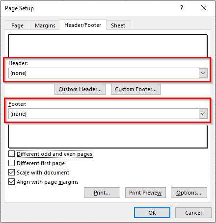
- Another way is to go to the ‘Page Setup’ dialog box and set it to ‘(None)‘, as shown below:
With this you have reached to the end of this blog. Share your thoughts, views, and comments in the comments section below.
RELATED POSTS
-
An Object in Excel – Create, Insert, Edit and Link
-
19 Everyday Use Excel VBA Codes
-
Start Automation – Record A Macro in Excel
-
Insert Symbols and Special Characters in Excel
-
How to Automatically Run a Macro when Workbook is Opened?
-
Add Macro to Quick Access Toolbar and Ribbon
How to Make Headers and Footers in Excel: Step-by-Step
Headers and footers in Excel are great for adding basic information to your worksheets such as page numbers, dates, or workbook names 😀
Adding headers or footers helps you add data without needing to change the data or format of your worksheet. This also makes your workbook look more professional when printed.
Unfortunately, header and footer tools in Excel are underused since it is a mystery for some Excel users 🔍
Let’s uncover that mystery and learn how you can insert headers and footers in Excel! Microsoft Excel offers you built-in headers and footers ready for use. Plus, you can even customize your own.
It’s easy. Let’s go!
Learn better by doing 👍 Make sure to download this free practice workbook we’ve prepared for you to work on.
How to add a header in Excel
A header is a text or image found on the top of each page of a document. Typically, a header is an area where you can insert document information like page numbers, document names, dates, and many more.
Inserting a header in Excel is simple. Open your practice workbook to insert one 😊
- Go to the Insert Tab.

- Click the Text Group.
- Select the Header & Footer button.

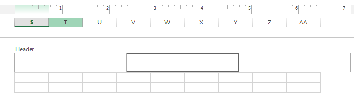
Once you click the Header and Footer button, the workbook view changes to the “Page Layout” view.
By default, the cursor is on the center section of the header box. But you can choose to write the header on either the left or right section boxes too.

Let’s try to type “Spreadsheeto.com” in the center section of the header like this.

Wasn’t that very easy? 😀
Add headers using preset headers
There are preset headers you can use in Excel. These preset headers are the most common elements you can insert in a header like Page Number, File Path or Name and so much more.
To do that, click “Header” on the left side of the Header & Footer Tab.

The preset header and footer tools already format text. You can choose which format you want the header text to look like.
Alternatively, you can choose preset elements for a header in the Header & Footer Elements group. You can see elements such as:
- Page number
- Number of pages
- Current date
- Current time
- File path
- File name
- Sheet name
- Picture

Let’s try to insert a header element into our current worksheet. For example, let’s insert “File Name” as our header 👇
- Click the center section of the header.
- Click File Name in the Header and Footer Elements.

When you click the File Name button, this will appear:
&[File]
- Click anywhere in your worksheet.
This is now the result. You added the document or file name as your header 👍

Using a preset or built-in header makes adding headers very easy! You didn’t have to manually type the file name into the section box.
Adding headers not only helps you elevate your content but also helps you save time from making templates as they will appear on every page of your document 😀
Pro Tip!
A well-thought header can get your audience engaged from the get-go. Engaging your reader is a priority if you want to be heard. And one of the effective ways to hook them is to have a great header in your reports and/or articles.
How to add a footer in Excel
A footer is just like a header but placed on the bottom of every document page. Footers are great for adding your contact information, links to CTAs or articles, page numbers, and more.
Just like adding headers, adding footers in Excel is easy too.
Insert a footer just like how you insert a header 👇
- Click Insert Tab in the Excel Ribbon.
- Click Text group.
- Select the Header & Footer.

- Click the “Go to Footer” icon on the Navigation group in the Ribbon.

When you click the “Go to Footer” icon, you will be directed to the footer part of the page.

Just like the header, the cursor is on the center section of the footer by default. If you would like to insert a footer on the left or right section, just click on them.
In these section boxes, you can type the footer information or use a preset footer in Excel 😊
Add footers using preset footers
The elements or presets used in headers can also be used in footers.
If you want the page number or the file name to be at the bottom of the page, insert it as footer information.
You can find them in the Header & Footer Elements group of the Header & Footer Tab.

Or go click the footer button to see footer presets.

You can choose to format text using preset footers in Excel.
Say, let’s add the Page Number in the footer.
- Click the center section of the footer.
- Click Page Number in the Header & Footer Elements.

When you click the Page Number button, this will appear:
&[Page]
- Click anywhere in your worksheet.
This is now the result. A page number is inserted as a footer in Excel 😀

Now, you don’t have to count and manually type the page number in your worksheet. Microsoft Excel does that for you using these header and footer tools.
Remember, adding headers and footers is not limited to just page numbers or file names. You can insert a date or time. You can insert a sheet or file path. You can also insert a picture 😉
But what if you changed your mind? How can you remove headers and footers in Excel? 🤔Well, lucky for you that’s what you are going to learn next!
How to remove headers and footers in Excel
Removing the headers or footers you’ve inserted is easy as well. You can remove headers and footers individually, or remove them at once.
Let’s delete the headers and footers we’ve inserted in our practice workbook all at once.
- Click the Page Layout Tab.
- In the Page Setup group, click the Page Setup dialog box launcher. It’s that little arrow.

When you click the page setup dialog box launcher, a page setup dialog box will pop up showing you a full set of page formatting options.
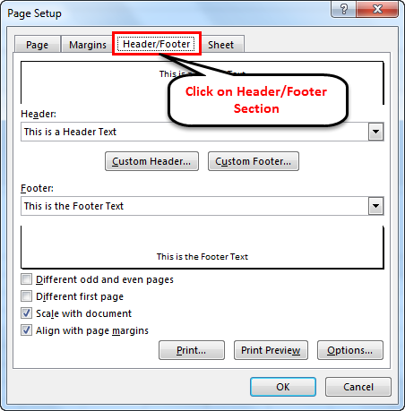
- Click the Header/Footer Tab in the Page Setup dialog box.

- Click the drop-down arrow and select “none” for the header.
- Do the same with the footer.
- Click OK.

By doing this, you removed all the headers and footers at once.
You can also remove headers and footers this way. But you have to remove the header and footer individually.
- Click on the Header section box.
- In the Header and Footer Tab, click Header.
- Click None.

The same way goes for footers. All you have to do is click on the footer text box, then click the Footer button in the Header and Footer Tab. Finally, click None to remove the footer.

It’s simple and easy, right?
Headers and footers are a staple function if you’re working on a multiple-paged article, newsletter, or worksheet 😊
That’s it – Now what?
Great job! You can now elevate your content by making it more organized and professional using Excel header and footer tools 🥳
You can, of course, create your own headers and footers or you can make Excel work for you by using built-in headers and footers. With only a few clicks, Excel built-in tools can help you save time and work.
Speaking of Excel’s built-in tools, you should get to learn Excel’s most powerful built-in tool: FUNCTIONS. Microsoft Excel provides you with a lot of built-in functions you can use to organize and calculate data in your spreadsheet 🚀
Learn the most essential functions that you (and everybody) actually need in daily work and life. Sign up for my free email course and learn about the IF, the SUMIF, and the VLOOKUP functions. You’ll also learn how to effectively clean your data in this email course 📧
Don’t miss out. It’s easy and free!
Frequently asked questions
A header is placed at the top of a page, while a footer is placed at the bottom, or foot, of a page. You can find the header and footer tools in Excel when you click the Insert Tab, and then click the Header & Footer button in the Text group.
Headers and footers are text placed on top and bottom of the page respectively. These are areas typically used to insert additional information about the document like page numbers, dates, file names, and more.
If you want to make a header only on the first page, click the header area on the first page. Go to the Header & Footer Tab that appears. In the Options group, check the Different First Page option box.
Kasper Langmann2023-01-09T20:47:55+00:00
Page load link
Header text often takes up too much space. Use these three formats to put headers on a diet when working in Excel.

In an ordinary sheet, descriptive header text often inflates the width of columns, pushing important data off screen. Moving from screen to screen is tedious and often, there’s nothing you can do about it. But, when the problem is the header text, you have choices. In this article, I’ll show you three cell formats that reduce the width of the header cells so you can get all of that data back on a single screen.
I’m using Office 365’s desktop version of Excel on a Windows 10 64-bit system, but you can apply these formats in older versions. You can use your own data or download the demonstration .xlsx and .xls files.
SEE: System update policy template download (Tech Pro Research)
Shrink to fit
Figure A shows an example of what often happens when header text exceeds the actual data in the column. What you can’t see is that the data range extends to column P–you’re missing a lot. You could use a smaller font size, or you could delete some of the header text, but there are better choices. You might consider Shrink to fit, but I admit that it’s my least favorite of the three formats.

To apply this format, select the header cells, B2:P2, and click the Alignment dialog launcher (on the Home tab). On the Alignment tab, check the Shrink to fit option shown in Figure B. Or, press Ctrl+1.

Figure C shows the results of reducing the width of column C–the effect is fairly dramatic. (You won’t see any difference until you reduce the width of the column.)

The text won’t increase if you increase the width of the column. In addition, the font size doesn’t actually change. If you check the Font Size control in the Font control, you’ll see that it’s the same as before. This format has limited use when fitting header text, but you should know it’s available.
Before continuing, be sure to remove the Shrink to fit format if you’re following along with the example because it’ll change the results of the next section, which introduces the Wrap Text format.
Wrap Text format
The Wrap Text format forces text to wrap to multiple lines within a single cell to accommodate the cell’s width. It’s easy to use, but this format sometimes yields unexpected results and requires a bit of tweaking.
Before applying the format, reduce the width of the column(s) to accommodate the text instead of the headers. Most of the header text will disappear. It’s temporary so don’t worry. Then, select the header cells, B2:P2, and click Wrap Text in the Alignment group on the Home tab.
As you can see in Figure D, you usually have to tweak a column or two–or maybe even all of them. Specifically, columns D and M need to be a bit wider to keep the words Membership and State together. This format won’t keep words together automatically. However, we can see all of the data on one screen now.

Sometimes you’ll want to rearrange the words a bit. Columns E, F, G, and H illustrate this possibility. You might want Last Name and First Name to be on the same line. When this happens, force a “hard return” in the header text. To do so, select the cell and position the cursor before the word (in the Formula bar) you want to push to the next line and press Alt+Enter. If you end up with three lines of header text, as shown in Figure E, simply increase the width of the column(s) a bit.

Most of the time, Wrap Text gets the job done, but there’s one more format you can try. If you’re following along, remove the Wrap Text format from the header cells (it’s a toggle, simply select the cells and click Wrap Text) and then increase the column widths so you can see the full text headers.
Orientation
If Wrap Text isn’t appropriate, try the Orientation format, which rotates the font angle. Select the header cells, B2:P2, and click Orientation in the Alignment group on the Home tab. Figure F shows the result of choosing Angle Counterclockwise from the drop-down list. Many users press Ctrl+z to undo the change and give up because it doesn’t help and it looks odd. But the truth is, you’re almost there. (The online version doesn’t support the cell Orientation format.)

Similarly to the Wrap Text function, the column width is part of the show. Figure G shows the result of reducing the column widths to accommodate the data instead of the headers.

This feature has a number of settings, so if you don’t like this one, change it. Press Ctrl+1 and adjust the angle using the Orientation control to the right. You can drag the text line up or down or enter a number in the Degree control. By default, the degree 45 is represented in both spots. Figure H shows the result of dragging the Text line to 75. To quickly remove the format, enter 0 in the Degree control.

Send me your question about Office
I answer readers’ questions when I can, but there’s no guarantee. Don’t send files unless requested; initial requests for help that arrive with attached files will be deleted unread. You can send screenshots of your data to help clarify your question. When contacting me, be as specific as possible. For example, “Please troubleshoot my workbook and fix what’s wrong” probably won’t get a response, but “Can you tell me why this formula isn’t returning the expected results?” might. Please mention the app and version that you’re using. I’m not reimbursed by TechRepublic for my time or expertise when helping readers, nor do I ask for a fee from readers I help. You can contact me at susansalesharkins@gmail.com.
See also
- How to use Word mail-merge (TechRepublic)
- Office Q&A: How to use a macro to set Find defaults (TechRepublic)
- How to use Office Picture Layout options to quickly arrange pictures (TechRepublic)
- How to use Excel’s find feature to highlight or delete matching values (TechRepublic)
- Office Q&A: How to share Outlook 365 contacts (TechRepublic)
- Office Q&A: How to anchor image files in Microsoft Word (TechRepublic)
- Microsoft Office 365 for business: Everything you need to know (ZDNet)