Format excel for dates - Word и Excel - помощь в работе с программами

Format a date the way you want

Excel for Microsoft 365 Excel for Microsoft 365 for Mac Excel for the web Excel 2021 Excel 2021 for Mac Excel 2019 Excel 2019 for Mac Excel 2016 Excel 2016 for Mac Excel 2013 Excel 2010 Excel 2007 Excel for Mac 2011 More…Less

When you enter some text into a cell such as «2/2″, Excel assumes that this is a date and formats it according to the default date setting in Control Panel. Excel might format it as «2-Feb». If you change your date setting in Control Panel, the default date format in Excel will change accordingly. If you don’t like the default date format, you can choose another date format in Excel, such as «February 2, 2012″ or «2/2/12″. You can also create your own custom format in Excel desktop.

Follow these steps:

Select the cells you want to format.
Press CTRL+1.
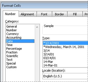
In the Format Cells box, click the Number tab.
In the Category list, click Date.
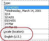
Under Type, pick a date format. Your format will preview in the Sample box with the first date in your data.

Note: Date formats that begin with an asterisk (*) will change if you change the regional date and time settings in Control Panel. Formats without an asterisk won’t change.
If you want to use a date format according to how another language displays dates, choose the language in Locale (location).

Tip: Do you have numbers showing up in your cells as #####? It’s likely that your cell isn’t wide enough to show the whole number. Try double-clicking the right border of the column that contains the cells with #####. This will resize the column to fit the number. You can also drag the right border of the column to make it any size you want.

If you want to use a format that isn’t in the Type box, you can create your own. The easiest way to do this is to start from a format this is close to what you want.

Select the cells you want to format.
Press CTRL+1.
In the Format Cells box, click the Number tab.
In the Category list, click Date, and then choose a date format you want in Type. You can adjust this format in the last step below.
Go back to the Category list, and choose Custom. Under Type, you’ll see the format code for the date format you chose in the previous step. The built-in date format can’t be changed, so don’t worry about messing it up. The changes you make will only apply to the custom format you’re creating.
In the Type box, make the changes you want using code from the table below.

To display	Use this code
Months as 1–12	m
Months as 01–12	mm
Months as Jan–Dec	mmm
Months as January–December	mmmm
Months as the first letter of the month	mmmmm
Days as 1–31	d
Days as 01–31	dd
Days as Sun–Sat	ddd
Days as Sunday–Saturday	dddd
Years as 00–99	yy
Years as 1900–9999	yyyy

If you’re modifying a format that includes time values, and you use «m» immediately after the «h» or «hh» code or immediately before the «ss» code, Excel displays minutes instead of the month.

To quickly use the default date format, click the cell with the date, and then press CTRL+SHIFT+#.
If a cell displays ##### after you apply date formatting to it, the cell probably isn’t wide enough to show the whole number. Try double-clicking the right border of the column that contains the cells with #####. This will resize the column to fit the number. You can also drag the right border of the column to make it any size you want.
To quickly enter the current date in your worksheet, select any empty cell, press CTRL+; (semicolon), and then press ENTER, if necessary.
To enter a date that will update to the current date each time you reopen a worksheet or recalculate a formula, type =TODAY() in an empty cell, and then press ENTER.

Follow these steps:

Select the cells you want to format.
Press Control+1 or Command+1.
In the Format Cells box, click the Number tab.
In the Category list, click Date.
Under Type, pick a date format. Your format will preview in the Sample box with the first date in your data.

Note: Date formats that begin with an asterisk (*) will change if you change the regional date and time settings in Control Panel. Formats without an asterisk won’t change.
If you want to use a date format according to how another language displays dates, choose the language in Locale (location).

If you want to use a format that isn’t in the Type box, you can create your own. The easiest way to do this is to start from a format this is close to what you want.

Select the cells you want to format.
Press Control+1 or Command+1.
In the Format Cells box, click the Number tab.
In the Category list, click Date, and then choose a date format you want in Type. You can adjust this format in the last step below.
Go back to the Category list, and choose Custom. Under Type, you’ll see the format code for the date format you chose in the previous step. The built-in date format can’t be changed, so don’t worry about messing it up. The changes you make will only apply to the custom format you’re creating.
In the Type box, make the changes you want using code from the table below.

To display	Use this code
Months as 1–12	m
Months as 01–12	mm
Months as Jan–Dec	mmm
Months as January–December	mmmm
Months as the first letter of the month	mmmmm
Days as 1–31	d
Days as 01–31	dd
Days as Sun–Sat	ddd
Days as Sunday–Saturday	dddd
Years as 00–99	yy
Years as 1900–9999	yyyy

To quickly use the default date format, click the cell with the date, and then press CTRL+SHIFT+#.
If a cell displays ##### after you apply date formatting to it, the cell probably isn’t wide enough to show the whole number. Try double-clicking the right border of the column that contains the cells with #####. This will resize the column to fit the number. You can also drag the right border of the column to make it any size you want.
To quickly enter the current date in your worksheet, select any empty cell, press CTRL+; (semicolon), and then press ENTER, if necessary.
To enter a date that will update to the current date each time you reopen a worksheet or recalculate a formula, type =TODAY() in an empty cell, and then press ENTER.

When you type something like 2/2 in a cell, Excel for the web thinks you’re typing a date and shows it as 2-Feb. But you can change the date to be shorter or longer.

To see a short date like 2/2/2013, select the cell, and then click Home > Number Format > Short Date. For a longer date like Saturday, February 02, 2013, pick Long Date instead.

If a cell displays ##### after you apply date formatting to it, the cell probably isn’t wide enough to show the whole number. Try dragging the column that contains the cells with #####. This will resize the column to fit the number.
To enter a date that will update to the current date each time you reopen a worksheet or recalculate a formula, type =TODAY() in an empty cell, and then press ENTER.

Need more help?

You can always ask an expert in the Excel Tech Community or get support in the Answers community.

Need more help?

Want more options?

Explore subscription benefits, browse training courses, learn how to secure your device, and more.

Communities help you ask and answer questions, give feedback, and hear from experts with rich knowledge.

Источник

Format numbers as dates or times

When you type a date or time in a cell, it appears in a default date and time format. This default format is based on the regional date and time settings that are specified in Control Panel, and changes when you adjust those settings in Control Panel. You can display numbers in several other date and time formats, most of which are not affected by Control Panel settings.

Display numbers as dates or times

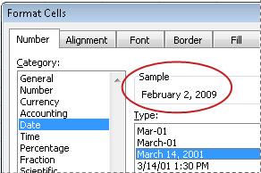
You can format dates and times as you type. For example, if you type 2/2 in a cell, Excel automatically interprets this as a date and displays 2-Feb in the cell. If this isn’t what you want—for example, if you would rather show February 2, 2009 or 2/2/09 in the cell—you can choose a different date format in the Format Cells dialog box, as explained in the following procedure. Similarly, if you type 9:30 a or 9:30 p in a cell, Excel will interpret this as a time and display 9:30 AM or 9:30 PM. Again, you can customize the way the time appears in the Format Cells dialog box.

On the Home tab, in the Number group, click the Dialog Box Launcher next to Number.

You can also press CTRL+1 to open the Format Cells dialog box.
In the Category list, click Date or Time.
In the Type list, click the date or time format that you want to use.

Note: Date and time formats that begin with an asterisk (*) respond to changes in regional date and time settings that are specified in Control Panel. Formats without an asterisk are not affected by Control Panel settings.
To display dates and times in the format of other languages, click the language setting that you want in the Locale (location) box.

The number in the active cell of the selection on the worksheet appears in the Sample box so that you can preview the number formatting options that you selected.

Top of Page

Create a custom date or time format

On the Home tab, click the Dialog Box Launcher next to Number.

You can also press CTRL+1 to open the Format Cells dialog box.
In the Category box, click Date or Time, and then choose the number format that is closest in style to the one you want to create. (When creating custom number formats, it’s easier to start from an existing format than it is to start from scratch.)
In the Category box, click Custom. In the Type box, you should see the format code matching the date or time format you selected in the step 3. The built-in date or time format can’t be changed or deleted, so don’t worry about overwriting it.
In the Type box, make the necessary changes to the format. You can use any of the codes in the following tables:

Days, months, and years

To display	Use this code
Months as 1–12	m
Months as 01–12	mm
Months as Jan–Dec	mmm
Months as January–December	mmmm
Months as the first letter of the month	mmmmm
Days as 1–31	d
Days as 01–31	dd
Days as Sun–Sat	ddd
Days as Sunday–Saturday	dddd
Years as 00–99	yy
Years as 1900–9999	yyyy

If you use «m» immediately after the «h» or «hh» code or immediately before the «ss» code, Excel displays minutes instead of the month.

Hours, minutes, and seconds

To display	Use this code
Hours as 0–23	h
Hours as 00–23	hh
Minutes as 0–59	m
Minutes as 00–59	mm
Seconds as 0–59	s
Seconds as 00–59	ss
Hours as 4 AM	h AM/PM
Time as 4:36 PM	h:mm AM/PM
Time as 4:36:03 P	h:mm:ss A/P
Elapsed time in hours; for example, 25.02	[h]:mm
Elapsed time in minutes; for example, 63:46	[mm]:ss
Elapsed time in seconds	[ss]
Fractions of a second	h:mm:ss.00

AM and PM If the format contains an AM or PM, the hour is based on the 12-hour clock, where «AM» or «A» indicates times from midnight until noon and «PM» or «P» indicates times from noon until midnight. Otherwise, the hour is based on the 24-hour clock. The «m» or «mm» code must appear immediately after the «h» or «hh» code or immediately before the «ss» code; otherwise, Excel displays the month instead of minutes.

Creating custom number formats can be tricky if you haven’t done it before. For more information about how to create custom number formats, see Create or delete a custom number format.

Top of Page

Tips for displaying dates or times

To quickly use the default date or time format, click the cell that contains the date or time, and then press CTRL+SHIFT+# or CTRL+SHIFT+@.
If a cell displays ##### after you apply date or time formatting to it, the cell probably isn’t wide enough to display the data. To expand the column width, double-click the right boundary of the column containing the cells. This automatically resizes the column to fit the number. You can also drag the right boundary until the columns are the size you want.
When you try to undo a date or time format by selecting General in the Category list, Excel displays a number code. When you enter a date or time again, Excel displays the default date or time format. To enter a specific date or time format, such as January 2010, you can format it as text by selecting Text in the Category list.
To quickly enter the current date in your worksheet, select any empty cell, and then press CTRL+; (semicolon), and then press ENTER, if necessary. To insert a date that will update to the current date each time you reopen a worksheet or recalculate a formula, type =TODAY() in an empty cell, and then press ENTER.

Need more help?

You can always ask an expert in the Excel Tech Community or get support in the Answers community.

Need more help?

Want more options?

Explore subscription benefits, browse training courses, learn how to secure your device, and more.

Communities help you ask and answer questions, give feedback, and hear from experts with rich knowledge.

Источник

One nice feature of Microsoft Excel is there’s usually more than one way to do many popular functions, including date formats. Whether you’ve imported data from another spreadsheet or database, or are merely entering due dates for your monthly bills, Excel can easily format most date styles.

Instructions in this article apply to Excel for Microsoft 365, Excel 2019, 2016, and 2013.

How to Change Excel Date Format Via the Format Cells Feature

With the use of Excel’s many menus, you can change up the date format within a few clicks.

Select the Home tab.
In the Cells group, select Format and choose Format Cells.
Under the Number tab in the Format Cells dialog, select Date.
As you can see, there are several options for formatting in the Type box.

You could also look through the Locale (locations) drop-down to choose a format best suited for the country you’re writing for.
Once you’ve settled on a format, select OK to change the date format of the selected cell in your Excel spreadsheet.

Make Your Own With Excel Custom Date Format

If you don’t find the format you want to use, select Custom under the Category field to format the date how you’d like. Below are some of the abbreviations you’ll need to build a customized date format.

Abbreviations used in Excel for Dates
Month shown as 1-12	m
Month shown as 01-12	mm
Month shown as Jan-Dec	mmm
Full Month Name January-December	mmmm
Month shown as the first letter of the month	mmmmm
Days (1-31)	d
Days (01-31)	dd
Days (Sun-Sat)	ddd
Days (Sunday-Saturday)	dddd
Years (00-99)	yy
Years (1900-9999)	yyyy

Select the Home tab.
Under the Cells group, select the Format drop-down, then select Format Cells.
Under the Number tab in the Format Cells dialog, select Custom. Just like the Date category, there are several formatting options.
Once you’ve settled on a format, select OK to change the date format for the selected cell in your Excel spreadsheet.

How to Format Cells Using a Mouse

If you prefer only using your mouse and want to avoid maneuvering through multiple menus, you can change the date format with the right-click context menu in Excel.

Select the cell(s) containing the dates you want to change the format of.
Right-click the selection and select Format Cells. Alternatively, press Ctrl+1 to open the Format Cells dialog.

Alternatively, select Home > Number, select the arrow, then select Number Format at the bottom right of the group. Or, in the Number group, you can select the drop-down box, then select More Number Formats.
Select Date, or, if you need a more customized format, select Custom.
In the Type field, select the option that best suits your formatting needs. This might take a bit of trial and error to get the right formatting.
Select OK when you’ve chosen your date format.

Whether using the Date or Custom category, if you see one of the Types with an asterisk (*) this format will change depending on the locale (location) you have selected.

Using Quick Apply for Long or Short Date

If you need a quick format change from to either a Short Date (mm/dd/yyyy) or Long Date (dddd, mmmm dd, yyyy or Monday, January 1, 2019), there’s a quick way to change this in the Excel Ribbon.

Select the cell(s) for which you want to change the date format.
Select Home.
In the Number group, select the drop-down menu, then select either Short Date or Long Date.

Using the TEXT Formula to Format Dates

This formula is an excellent choice if you need to keep your original date cells intact. Using TEXT, you can dictate the format in other cells in any foreseeable format.

To get started with the TEXT formula, go to a different cell, then enter the following to change the format:

=TEXT(##, “format abbreviations”)

## is the cell label, and format abbreviations are the ones listed above under the Custom section. For example, =TEXT(A2, “mm/dd/yyyy”) displays as 01/01/1900.

Using Find & Replace to Format Dates

This method is best used if you need to change the format from dashes (-), slashes (/), or periods (.) to separate the month, day, and year. This is especially handy if you need to change a large number of dates.

Select the cell(s) you need to change the date format for.
Select Home > Find & Select > Replace.
In the Find what field, enter your original date separator (dash, slash, or period).
In the Replace with field, enter what you’d like to change the format separator to (dash, slash, or period).
Then select one of the following:
- Replace All: Which will replace all the first field entry and replace it with your choice from the Replace with field.
- Replace: Replaces the first instance only.
- Find All: Only finds all of the original entry in the Find what field.
- Find Next: Only finds the next instance from your entry in the Find what field.

Using Text to Columns to Convert to Date Format

If you have your dates formatted as a string of numbers and the cell format is set to text, Text to Columns can help you convert that string of numbers into a more recognizable date format.

Select the cell(s) that you want to change the date format.
Make sure they are formatted as Text. (Press Ctrl+1 to check their format).
Select the Data tab.
In the Data Tools group, select Text to Columns.
Select either Delimited or Fixed width, then select Next.

Most of the time, Delimited should be selected, as date length can fluctuate.
Uncheck all of the Delimiters and select Next.
Under the Column data format area, select Date, choose the format your date string using the drop-down menu, then select Finish.

Using Error Checking to Change Date Format

If you’ve imported dates from another file source or have entered two-digit years into cells formatted as Text, you’ll notice the small green triangle in the top-left corner of the cell.

This is Excel’s Error Checking indicating an issue. Because of a setting in Error Checking, Excel will identify a possible issue with two-digit year formats. To use Error Checking to change your date format, do the following:

Select one of the cells containing the indicator. You should notice an exclamation mark with a drop-down menu next to it.
Select the drop-down menu and select either Convert XX to 19XX or Convert xx to 20XX, depending on the year it should be.
You should see the date immediately change to a four-digit number.

Using Quick Analysis to Access Format Cells

Quick Analysis can be used for more than formatting the color and style of your cells. You can also use it to access the Format Cells dialog.

Select several cells containing the dates you need to change.
Select Quick Analysis in the lower right of your selection, or press Ctrl+Q.
Under Formatting, select Text That Contains.
Using the right drop-down menu, select Custom Format.
Select the Number tab, then select either Date or Custom.
Select OK twice when complete.

Thanks for letting us know!

Get the Latest Tech News Delivered Every Day

Источник

What is a date in Excel?

A date is a number! And like any number (currency, percentage, decimal, …), you can customize your date format 👍

Dates are whole numbers

Usually, when you insert a date in a cell it is displayed in the format dd/mm/yyyy or mm/dd/yyyy.

Let’s say you have the date 01/01/2016 in a cell. If you change the cell’s format to Standard, the cell displays 42370 😕🤔

Explanation of the numbering

In Excel, a date is the number of days since 01/01/1900 (the first date in Excel).

So 42370 is the number of days between 01/01/1900 and 01/01/2016.

Date format

Dates can be displayed in different ways using the following 2 options (available in the Number Format dropdown in the main menu):

Short Date
Long Date

How to customize a date?

To customize a date:

Open the dialog box Custom Number (with the shortcut Ctrl + 1 or by clicking on the menu More number formats at the bottom of the number format dropdown)

In this dialog box, you select ‘Custom‘ in the Category list and write the date format code in ‘Type‘.

To format a date, you just write the parameter d, m or y a different number of times. For example,

dd/mm/yyyy will display 01/01/2016
dd mmm yyyy => 01 Jan 2016
mmmm yyyy => January 2016
dddd dd => Friday 01

In function of your language , the letter could be different:

t for «tag» (day) in German
j for «jour» (day) in French
a for «año» (year) in Spanish

Don’t write text in your cell !!!

With dates, one of the most common mistakes is to write text inside the format code (1 January 2016 for example). Never do this in Excel ⛔⛔⛔

If you do this, the contents of the cell will be Text and not a number

In Excel, text is always displayed on the left of a cell.
A number or a date is displayed on the right.

If you want to display the month in letters, just change the month format of your date.

Different examples of custom date

The following document shows you the same date but in different formats. The code for each date is in column A.

Different writing of dates according to the format code

In the following document, you can see the impact of each format on the same date.

Источник

In this guide, we’ll learn how to change date format in Excel. Date and Time data is an integral part of any statistical document or sheet. It is important to accurately track and analyze events, sales, figures, and others.

By convention, Excel uses a general data format that may be as per your need. But in most cases, that format may need to be customized.

Changing the format of Date in a particular cell or all the cells in your Excel sheet is an easy process and doesn’t require any complex methodologies. Excel provides a wide range of formatting options based on Location and Languages which helps in better date formatting in native language and style. Also, For some Languages there is also features to select from different Calendar types.

Follow the below step-by-step tutorial to change date format in Excel quickly and easily.

Step 1. Select the range of cells containing the date

To start with, select the cell values where want to change the date format, as shown in the image below.

Sample selection of dates in default formatting option

Step 2. Go to Number Format dropdown

To select ‘Number Format’, go to ‘Home‘ in the option menu and look for Number Format, as shown below
Then from the drop-down menu, select ‘More Number Formats‘ to reveal the ‘Number Format’ dialogue menu.

Select Number Format

Alternatively, you may directly go to Number Format, by right-clicking on the selected cell/s
Click on ‘Number Format’.

Right Click and select Number Format

Step 3. Choose Date

From the Category menu on the right, choose ‘Date‘.

Format Date option menu

Now, to apply any date formatting type, select it from the right panel of the pop-up menu of Number Format. Click on ‘OK‘ to apply the formatting to the selected cell/s.

Note: You may check the date format implementation in the ‘Sample‘ at the top of the menu option

Choose the Date Type

The general option type to choose from a variety of Date Formatting options. Scroll down in this section to reveal a plethora of options for formatting, ranging from date, text (month name), year, and others.

This option can be perceived as the display menu, as the formatting options in this will keep on changing as per the selection in Locale(Location) and Calendar type.

General Date Formatting

Choose the Locale (location)

This option features the Location or Language options to help format the date accordingly. This option is probably the most used option as users require to format the date according to their or audience preference as per the native formatting style, based on language and location.

Choose any language or Location from this options menu. After selecting, all the supported date format options available for that particular locale will be available for selecting in the above Type menu.

selecting locale (language) in date formatting

Choose the type of calendar

This option reveals different calendar types available based on the Locale(Location) selected from the above option menu. This formatting option is only available for certain Locale and not all.

As shown in our example below, the variety of calendar types available for selection are only available for the Locale (location) selected (here, Arabia), for other locales the calendar type might be different or not at all present.

Selecting Calendar type in Date Formatting

To apply selected formatting, you will need to click ‘OK‘ after selection to apply to your dates.

Conclusion

That’s It! You can now easily convert your dates to your desired format style easily.

We hope you learned and enjoyed this lesson and we’ll be back soon with another awesome Excel tutorial at QuickExcel!

Источник

Need more help?

Need more help?

Want more options?

In this article

Display numbers as dates or times

Create a custom date or time format

Tips for displaying dates or times

Need more help?

Need more help?

Want more options?

How to Change Excel Date Format Via the Format Cells Feature

Make Your Own With Excel Custom Date Format

How to Format Cells Using a Mouse

Using Quick Apply for Long or Short Date

Using the TEXT Formula to Format Dates

Using Find & Replace to Format Dates

Using Text to Columns to Convert to Date Format

Using Error Checking to Change Date Format

Using Quick Analysis to Access Format Cells

What is a date in Excel?

Dates are whole numbers

Explanation of the numbering

Date format

How to customize a date?

Don’t write text in your cell !!!

Different examples of custom date

Different writing of dates according to the format code

Step 1. Select the range of cells containing the date

Step 2. Go to Number Format dropdown

Step 3. Choose Date

Choose the Date Type

Choose the Locale (location)

Choose the type of calendar

Conclusion