
Create and format tables
Create and format a table to visually group and analyze data.
Note: Excel tables shouldn’t be confused with the data tables that are part of a suite of What-If Analysis commands (Forecast, on the Data tab). See Introduction to What-If Analysis for more information.

Try it!
-
Select a cell within your data.
-
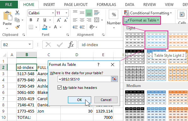
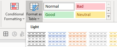
Select Home > Format as Table.
-
Choose a style for your table.
-
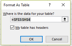
In the Create Table dialog box, set your cell range.
-
Mark if your table has headers.
-
Select OK.
-
Insert a table in your spreadsheet. See Overview of Excel tables for more information.
-
Select a cell within your data.
-
Select Home > Format as Table.
-
Choose a style for your table.
-
In the Create Table dialog box, set your cell range.
-
Mark if your table has headers.
-
Select OK.
To add a blank table, select the cells you want included in the table and click Insert > Table.
To format existing data as a table by using the default table style, do this:
-
Select the cells containing the data.
-
Click Home > Table > Format as Table.
-
If you don’t check the My table has headers box, Excel for the web adds headers with default names like Column1 and Column2 above the data. To rename a default header, double-click it and type a new name.
Note: You can’t change the default table formatting in Excel for the web.
Want more?
Overview of Excel tables
Video: Create and format an Excel table
Total the data in an Excel table
Format an Excel table
Resize a table by adding or removing rows and columns
Filter data in a range or table
Convert a table to a range
Using structured references with Excel tables
Excel table compatibility issues
Export an Excel table to SharePoint
Need more help?
Formatting cells as a table this is a process, that requires a lot of time, but that brings little benefit. A lot of effort can be saved by using ready-made styles of table layout.
Let`s descry ready-made designer stylish solutions that are predefined in the Excel tool set. You can also think about creating and maintaining your own styles. For this purpose, the program provides for special tools and tools.
How to create and format as a table in Excel?
We format the original range from the previous lessons with the helping of style design.
- Move the cursor to any cell in the table within the range A1:D4.
- Select the «Format as Table» tool on the «HOME» tab, the «Styles» section. There are the wide selection of ready-made and harmonious in design styles before you . Specify the style «Style Light 2». The dialog box appears where the range of the table data location is determined. Do not change anything, pressing OK.
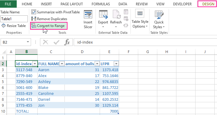
- The table has completely changed into a new and stylish format. There are even added filter control buttons. And on the broad band of tools the bookmark «DESIGN» was added, above which the inscription «TABLES TOOLS» is highlighted.
- To remove all unnecessary from our table and leave only the format, go to the «Designer» tab and in the «Tools» section, select «Convert to Range». Press OK to confirm.
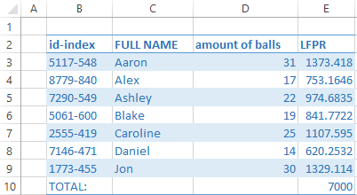
The notation. Note, that Excel itself recognized to the size of the table, we did not need to allocate a range, it was enough to specify one of any cells.
Although there are a lot of styles, sometimes you can not find the right one. To save time, you should choose the most similar style and format it for your needs.
To clear the format, you must first select the required range of cells and select the tool on the «HOME tab» – «Editing» – «Clear Formats». For quick removal only of the cell boundaries, use the shortcut key combination CTRL + SHIFT + (minus). Just do not forget to select the range before that.
Convert Data Into a Table in Excel
This page will show you how to convert Excel data into a table.
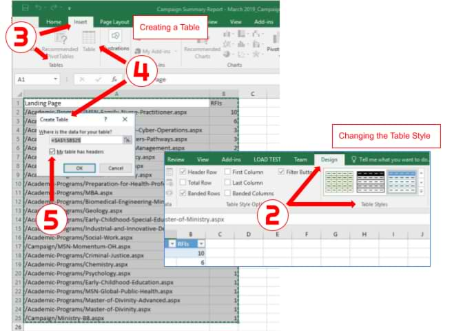
Creating a Table within Excel
- Open the Excel spreadsheet.
- Use your mouse to select the cells that contain the information for the table.
- Click the «Insert» tab > Locate the «Tables» group.
- Click «Table». A «Create Table» dialog box will open.
- If you have column headings, check the box «My table has headers».
- Verify that the range is correct > Click [OK].
- Resize your columns to make the headings visible.
Changing the Table Style
- Click on a cell in the table to activate the «Table Tools» tab.
- Click the «Design» tab > Locate the «Table Styles» group.
- Choose a style/color option that appeals to you. (Hover over the various table styles to see a live preview.)
Keywords: Office, color, colors, filter, sort, rows, columns, apply, enhance, table
Share This Post
-
Facebook
-
Twitter
-
LinkedIn
Blog Resources
Cedarville offers more than 150 academic programs to grad, undergrad, and online students. Cedarville is known for its biblical worldview, academic excellence, intentional discipleship, and authentic Christian community.

Loading…
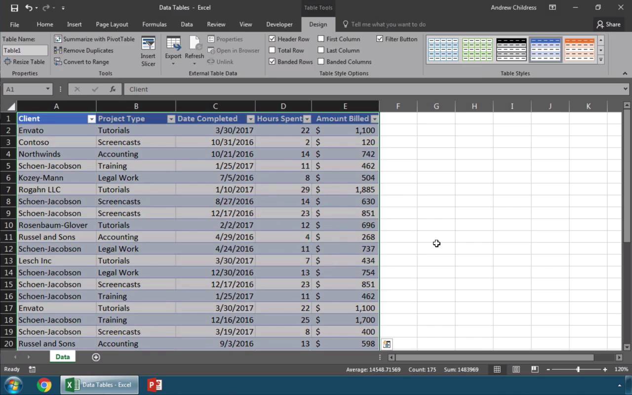
In just 60 seconds, I’ll show you a couple of features that will really help you see the power of using tables in Microsoft Excel.
How to Quickly Make Data Tables in Excel
Note: Watch this short tutorial screencast or follow the quick steps below, that compliment this video.
1. Format Our Data as a Table in Excel
So, right now I have a regular set of data here in Excel, and we’ll start off by converting it into a table. Let’s make sure that we’re on the Home tab of the Excel ribbon and that we’ve clicked anywhere inside the data. Let’s find the Format as Table button.


2. Apply a Table Style to Our Excel Data
When I click on it, the first advantage is that we can choose a style we like and apply it to the table. Let’s choose one of these and click on it. We get this pop up box that just double checks that we have our data selected, and I’ll press OK for now.


3. Filter Data Tables and Make Clean Excel Formulas
You can see that the style is applied, but there’s more too. At the top, we now have easy filters for data. So I can click on one to change the filter. Let’s also say that we wanna add a new column, a calculation on the far right side. I’ll give it a title and then write my formula here right below it.


Finishing Up!
You can see that the formula is much cleaner and simpler, and when I enter it, it writes it for every cell in that column. The table expands as well, to include this new column. These are just a couple of the reasons to use tables in your Excel spreadsheets.
More Great Excel Tutorials on Envato Tuts+
Find comprehensive Excel tutorials on Envato Tuts+ to help you learn how to work with your data better in your spreadhsheets. We also have a quick-start in 60 seconds Excel video series to learn more Excel tools fast.
Here are a few Excel tutorials to jump into to now:
Remember: Every Microsoft Excel tool you learn, and workflow you master, the more powerful spreadsheets you’ll make.
Purpose: to create, rename and format Excel Tables.
Creating an Excel Table turns a simple grid or matrix of data into a structured object which has many useful properties.
The ‘Format as Table‘ options are on the Home tab of Excel’s ribbon, next to the ‘Conditional Formatting’ options.
Links to topics on this page
- 10 benefits to using tables in Excel
- To format a range of cells as a table
- Resize an Excel Table
- Rename a table in Excel
- Add ‘Change Table Name’ to the Quick Access Toolbar
- To add totals and other summary data and functions to a table in Excel
- Using a form for data entry into a table
10 benefits to using Tables in Excel
- A table in Excel automatically expands when new rows or columns are added, so formulas or charts referencing the table will update dynamically;
- Easy to create a pivot table — click in any cell in the table, and select Insert | Pivot table from the ribbon;
- Add slicers — you may be familiar with using slicers with pivot tables; you can also use them in tables. Select ‘Insert slicer‘ from the Table Design tab in the ribbon;
- Auto-filling columns — change the formula in any cell, and the whole column will update (with the easy option to NOT auto-populate the column if you don’t want it);
- Totals and other summary functions are easy to add (see details below);
- Use a data entry form to add data (see details below);
- Structured referencing makes it easier to build, read and check formulas;
- There are lots of styles to choose from the style selector, and table styling automatically updates as the table expands. It’s also easy to change the style of the whole table, or create your own custom style;
- Ranges within the table are automatically named;
- Sorting and filtering are automatically activated in an Excel Table.
To format a range of cells as a table
- Select the range of cells to be turned into a table.
- Select ‘Format as Table‘ from the Home tab in the ribbon.
- In the dialog box that opens, tick the box ‘My table has headers‘ if your range of cells contains a column header row. If you don’t already have column headers, Excel will automatically add ‘Column1’, ‘Column2’, ‘Column3’, etc. You can easily amend column headers.
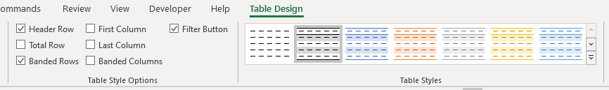
- Select the desired styling from the table design options.
When a table is created or being amended, the ‘Table Design‘ tab in Excel’s ribbon will automatically appear.
If you paste data into a worksheet in Excel, the range is highlighted, and you can select ‘Format as Table’ straightaway, without having to re-select the data (very helpful with a large set of data).
Resize an Excel Table
An Excel Table will automatically add new rows and columns as you add new data adjacent to the existing table boundaries.
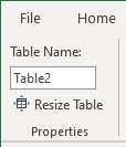
However, you may wish to make manual adjustments to the table, which you can do via the ‘Properties‘ section on the ‘Table Design‘ tab on the ribbon.
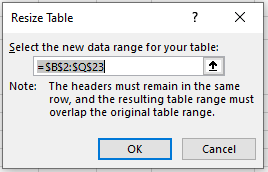
Select ‘Resize Table‘ from Properties, and the Resize Table dialog box opens. An adjustable border surrounds the existing table, and the new range can be set via the Select new data range box.
Note that Excel alerts you to the fact that the headers must remain in the same row, and the resulting table range must overlap the original table range (i.e. contain at least some of the header row and cell range of the existing table).
Rename a table in Excel
When tables are created, Excel will automatically name them ‘Table1’, ‘Table2’, ‘Table3’ etc.
Rename tables to something more useful via the ‘Properties‘ section of the Table Design tab of Excel’s ribbon.
Customize the Quick Access Toolbar in Excel to include the ‘Change Table Name’ command
Right-click ‘Table Name’ in the ‘Properties’ section of the Table Design tab, and select ‘Add to Quick Access Toolbar‘. If you’re working with several tables within a workbook, it’s handy to always be able to view the name of the current table you’re working in.
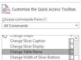
You can also add it to the list of commands, and place it in the order you want in the QA toolbar, via the ‘Customize the Quick Access Toolbar’ options.
See more options on customizing the ribbon in Excel in our topic page.
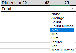
To add totals and other summary data and functions to a table in Excel
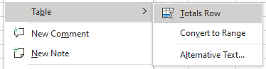
- Right-click any cell in the table, and select Table | Totals Row.
- An additional row will be added to the bottom of the table, and each column can be summarized (total, average, count, min, max, etc.) using the dropdown arrow in the bottom cell.
Using a form for data entry into a table
- Note: the ‘Form’ command in Excel isn’t on the ribbon by default, so you’ll need to add it — see our page on how to customize the ribbon in Excel.
- Select ‘Form‘ from the ribbon or Quick Access Toolbar.
- See our page on how to create a data entry form in Excel and enter or amend data.