
При необходимости Вы можете легко добавить к стандартным числовым форматам Excel свои собственные. Для этого выделите ячейки, к которым надо применить пользовательский формат, щелкните по ним правой кнопкой мыши и выберите в контекстном меню команду Формат ячеек (Format Cells) — вкладка Число (Number), далее — Все форматы (Custom):

В появившееся справа поле Тип: введите маску нужного вам формата из последнего столбца этой таблицы:

Как это работает…
На самом деле все очень просто. Как Вы уже, наверное, заметили, Excel использует несколько спецсимволов в масках форматов:
- 0 (ноль) — одно обязательное знакоместо (разряд), т.е. это место в маске формата будет заполнено цифрой из числа, которое пользователь введет в ячейку. Если для этого знакоместа нет числа, то будет выведен ноль. Например, если к числу 12 применить маску 0000, то получится 0012, а если к числу 1,3456 применить маску 0,00 — получится 1,35.
- # (решетка) — одно необязательное знакоместо — примерно то же самое, что и ноль, но если для знакоместа нет числа, то ничего не выводится
- (пробел) — используется как разделитель групп разрядов по три между тысячами, миллионами, миллиардами и т.д.
- [ ] — в квадратных скобках перед маской формата можно указать цвет шрифта. Разрешено использовать следующие цвета: черный, белый, красный, синий, зеленый, жёлтый, голубой.
Плюс пара простых правил:
- Любой пользовательский текст (кг, чел, шт и тому подобные) или символы (в том числе и пробелы) — надо обязательно заключать в кавычки.
- Можно указать несколько (до 4-х) разных масок форматов через точку с запятой. Тогда первая из масок будет применяться к ячейке, если число в ней положительное, вторая — если отрицательное, третья — если содержимое ячейки равно нулю и четвертая — если в ячейке не число, а текст (см. выше пример с температурой).
Ссылки по теме
- Как скрыть содержимое ячейки с помощью пользовательского формата
Excel for Microsoft 365 for Mac Excel 2021 for Mac Excel 2019 for Mac Excel 2016 for Mac Excel for Mac 2011 More…Less
If a built-in number format does not meet your needs, you can create a new number format that is based on an existing number format and add it to the list of custom number formats. For example, if you’re creating a spreadsheet that contains customer information, you can create a number format for telephone numbers. You can apply the custom number format to a string of numbers in a cell to format them as a telephone number.
Important: Custom number formats affect only the way a number is displayed and do not affect the underlying value of the number. Custom number formats are stored in the active workbook and are not available to new workbooks that you open.
Create a custom number format
-
On the Home tab, in the Number group, click More Number Formats at the bottom of the Number Format list
 .
. -
In the Format Cells dialog box, under Category, click Custom.
-
In the Type list, select the built-in format that most resembles the one that you want to create. For example, 0.00.
The number format that you select appears in the Type box.
-
In the Type box, modify the number format codes to create the exact format that you want. For example, 000-000-0000.
Your changes will not alter the built-in format. Instead, your changes create a new custom number format.
-
When you have finished, click OK.
Apply a custom number format
-
Select the cell or range of cells that you want to format.
-
On the Home tab, in the Number group, click More Number Formats at the bottom of the Number Format list
. -
In the Format Cells dialog box, under Category, click Custom.
-
At the bottom of the Type list, select the built-in format that you just created. For example, 000-000-0000.
The number format that you select appears in the Type box.
-
Click OK.
Delete a custom number format
-
On the Home tab, in the Number group, click More Number Formats at the bottom of the Number Format list
. -
In the Format Cells dialog box, under Category, click Custom.
-
In the Type list, select the custom number format, and then click Delete.
Notes:
-
Built-in number formats cannot be deleted.
-
Any cells in the workbook that were formatted with the deleted custom format will be displayed in the default General format.
-
Create a custom number format
-
On the Home tab, under Number, on the Number Format pop-up menu
, click Custom. -
In the Format Cells dialog box, under Category, click Custom.
-
In the Type list, select the built-in format that most resembles the one that you want to create. For example, 0.00.
The number format that you select appears in the Type box.
-
In the Type box, modify the number format codes to create the exact format that you want. For example, 000-000-0000.
Your changes will not alter the built-in format. Instead, your changes create a new custom number format.
-
When you have finished, click OK.
Apply a custom number format
-
Select the cell or range of cells that you want to format.
-
On the Home tab, under Number, on the Number Format pop-up menu
, click Custom. -
In the Format Cells dialog box, under Category, click Custom.
-
At the bottom of the Type list, select the built-in format that you just created. For example, 000-000-0000.
The number format that you select appears in the Type box.
-
Click OK.
Delete a custom number format
-
On the Home tab, under Number, on the Number Format pop-up menu
, click Custom. -
In the Format Cells dialog box, under Category, click Custom.
-
In the Type list, select the custom number format, and then click Delete.
Notes:
-
Built-in number formats cannot be deleted.
-
Any cells in the workbook that were formatted with the deleted custom format will be displayed in the default General format.
-
See also
Number format codes
Display dates, times, currency, fractions, or percentages
Highlight patterns and trends with conditional formatting
Display or hide zero values
Display numbers as postal codes, Social Security numbers, or phone numbers
Need more help?
Learning how to customise a cell format in Excel allows you to not only format your data the way you want, but in some instances it can save you time.
Before we dive in you need to know that despite how the text appears after you’ve set your custom cell format, the underlying value is unchanged for the purpose of formulas and calculations.
How to enter an Excel custom cell format
Select the cell/s you want to format then open the Format Cells window.
- The quick way just press CTRL+1
- Or the way most people do it is to right click and select ‘Format Cells’.
- On the Number Tab select Custom from the Category list.

Note: It’s handy to have the text you want to format in the cell before you press CTRL+1 because Excel will give you a sample view of what the text is going to look like in the Format Cells window, so you can see before pressing OK, if it’s what you want.
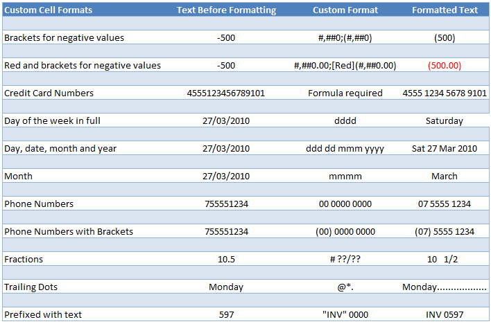
How to make your cell formats look the way you want
| Custom Cell Formats | Text Before Formatting | Custom Format | Formatted Text |
| Brackets for negative values | -500 | #,##0;(#,##0) | (500) |
| Red and brackets for negative values | -500 | #,##0.00;[Red](#,##0.00) | (500.00) |
| Day of the week in full | 27/03/2010 | dddd | Saturday |
| Day, date, month and year | 27/03/2010 | ddd dd mmm yyyy | Sat 27 Mar 2010 |
| Month | 27/03/2010 | mmmm | March |
| Phone Numbers | 755551234 | 00 0000 0000 | 07 5555 1234 |
| Phone Numbers with Brackets | 755551234 | (00) 0000 0000 | (07) 5555 1234 |
| Fractions | 10.5 | # ??/?? | 10 1/2 |
How to save time with Custom Cell Formats
1) From time to time I create a reference sheet like a contacts list, an index or even just a list of items like the one below using the custom cell format @*.

Because the text in the first column is often different lengths it can be hard for the eye to follow across. In these cases I like to use trailing dots to help the reader.
I wouldn’t dream of manually entering the dots but since I can create a custom format it’s worth it, plus I think it looks more elegant that using borders for this purpose as they can get a bit busy.
The custom cell format for trailing dots is @*. When you type in your text Excel will automatically enter the dots to fill to the end of the cell.
Tip: You’re not just limited to dots. You can have —- or **** or ____ or almost anything you want. Just replace the dot in the custom format with the character of your choice.
2) The other custom format I use regularly is prefixing my data with text. For example, I keep a record of our invoices and instead of typing ‘INV’ before each number I enter I use a custom cell format like this: “INV” 0000
Then when I type in 597 Excel converts it to INV 0597.
Tip: Replace INV with different text to suit your needs. It might be PO for purchase order, or any other text you can think of. Or make the text a suffix by changing the custom format to 0000 «INV».
Remember that even though the text appears to be INV 0597, for the purpose of formulas it’s still just a number 597.

Formatting cells for credit card numbers
You might be thinking you can use a custom format of 0000 0000 0000 0000 for credit card numbers, but you’ll find that it will only work for cards where the last number of the card is a zero! Try it out and see for yourself.
The workaround is to use a formula. This requires entering the number in one cell, and then in another cell you need to enter the following formula (assuming our credit card number is in cell A1):
=LEFT(A1,4) & " " & MID(A1,5,4) & " " & MID(A1,9,4) & " " & RIGHT(A1,4)
Note: I’ve added spaces in the formula for clarity.
Some explanation:
- The LEFT, MID and RIGHT returns text from a specified position in a cell.
- The ampersands ‘&’ join text together
- The “ “ adds a space between each group of text
[UPDATE] — You can also use this custom number format for credit cards and long phone numbers:
[<=99999999999]##########;#### #### #### ####
Thanks to MF for sharing that tip.
Enter your email address below to download the sample workbook.
By submitting your email address you agree that we can email you our Excel newsletter.
Excel includes a variety of built-in formats that cover general, numeric, currency, percentage, exponential, date, time, and custom numeric formats. You can also design custom formats based on one of the built-in formats.

To define a custom format, follow these steps:
1. Enter sample text for the format in a cell, and then select that cell (Excel then displays the sample text in the new format, which helps see the effects of your changes).
2. Do one of the following:
- Right-click on the selection and choose Format Cells… in the popup menu:

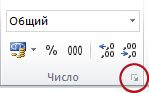
- On the Home tab, in the Number group, click the dialog box launcher:

- Press Ctrl+1.

3. In the Format Cells dialog box:
- On the Number tab, in the Category box, select the Custom item:

- In the Type list box, select the custom format you want to base your new custom format. Excel displays the details for the type in the Type text box.
- If the details for the type extend beyond the Type text box, double-click in the Type text box to select all its contents, issue a Copy command (for example, press Ctrl+C), and then paste the copied text into a text editor, such as Notepad. (For a shorter type, you can work effectively in the Type text box. For a longer type, it’s easier to have enough space to see the whole type at once.)
- Enter the details for the four parts of the type, separating the
parts from each other with a semicolon:- If you write formats with conditions such as [< 1000] and [≥ 1000], the format for the calculated condition is applied,
- Otherwise:
- If you write two formats, the first applies to positive and zero values and the second applies to negative values
- If you write three formats, the first applies to positive values, the second to negative values, and the third to zero
- If you write four formats, they apply to positive, negative, zero, and text values, respectively:
<positive>; <negative>; [zero]; [text]
- If you’re working in a text editor, copy what you typed and paste it
into the Type text box. Check the sample text to make sure it seems to be correct. - Click the OK button.

Codes for custom number formats
| Code | Description |
|---|---|
| General | Displays the number in general format. |
| # | Displays only significant digits and does not display insignificant zeros. |
| 0 (zero) | Displays insignificant zeros if a number has fewer digits than the zeros in the format. |
| ? | Displays a space for insignificant zeros on either side of the decimal point so that the decimal points align when formatted in a fixed-width font.
It can also be used for fractions with different numbers of digits. |
| . | Decimal point. |
| % | Percent symbol. |
| , | Thousand separator. |
| E-, E+, e-, e+ | Scientific notation. |
| $, —, +, /, (, ), :, space | Displays this character. |
| * | Repeats the next character to fill the full width of the column:
|
| _ (underscore) | Leaves a space equal to the width of the next character. |
| “text” | Displays text enclosed in double quotes. |
| @ | Text placeholder. |
| [color] | Displays characters in the specified color – black, blue, cyan, green, magenta, red, white , or yellow . |
| [condition value] | Custom criteria for each number format section. |

See also this tip in French:
Format de cellule personnalisé.
Please, disable AdBlock and reload the page to continue
Today, 30% of our visitors use Ad-Block to block ads.We understand your pain with ads, but without ads, we won’t be able to provide you with free content soon. If you need our content for work or study, please support our efforts and disable AdBlock for our site. As you will see, we have a lot of helpful information to share.
Содержание
- Create and apply a custom number format
- Create a custom number format
- Apply a custom number format
- Delete a custom number format
- Create a custom number format
- Apply a custom number format
- Delete a custom number format
- Создание пользовательского числового формата
- Дополнительные сведения
- Custom Excel number format
- How to create a custom number format in Excel
- Understanding Excel number format
- Excel formatting rules
- Digit and text placeholders
- Excel formatting tips and guidelines
- How to control the number of decimal places
- How to show a thousands separator
- Round numbers by thousand, million, etc.
- Text and spacing in custom Excel number format
- Including currency symbols in a custom number format
- How to display leading zeros with Excel custom format
- Percentages in Excel custom number format
- Fractions in Excel number format
- Create a custom Scientific Notation format
- Show negative numbers in parentheses
- Display zeroes as dashes or blanks
- Add indents with custom Excel format
- Change font color with custom number format
- Repeat characters with custom format codes
- How to change alignment in Excel with custom number format
- Apply custom number formats based on conditions
- Dates and times formats in Excel
Create and apply a custom number format
If a built-in number format does not meet your needs, you can create a new number format that is based on an existing number format and add it to the list of custom number formats. For example, if you’re creating a spreadsheet that contains customer information, you can create a number format for telephone numbers. You can apply the custom number format to a string of numbers in a cell to format them as a telephone number.
Important: Custom number formats affect only the way a number is displayed and do not affect the underlying value of the number. Custom number formats are stored in the active workbook and are not available to new workbooks that you open.
Create a custom number format
On the Home tab, in the Number group, click More Number Formats at the bottom of the Number Format list  .
.
In the Format Cells dialog box, under Category, click Custom.
In the Type list, select the built-in format that most resembles the one that you want to create. For example, 0.00.
The number format that you select appears in the Type box.
In the Type box, modify the number format codes to create the exact format that you want. For example, 000-000-0000.
Your changes will not alter the built-in format. Instead, your changes create a new custom number format.
When you have finished, click OK.
Apply a custom number format
Select the cell or range of cells that you want to format.
On the Home tab, in the Number group, click More Number Formats at the bottom of the Number Format list .
In the Format Cells dialog box, under Category, click Custom.
At the bottom of the Type list, select the built-in format that you just created. For example, 000-000-0000.
The number format that you select appears in the Type box.
Delete a custom number format
On the Home tab, in the Number group, click More Number Formats at the bottom of the Number Format list .
In the Format Cells dialog box, under Category, click Custom.
In the Type list, select the custom number format, and then click Delete.
Built-in number formats cannot be deleted.
Any cells in the workbook that were formatted with the deleted custom format will be displayed in the default General format.
Create a custom number format
On the Home tab, under Number, on the Number Format pop-up menu , click Custom.
In the Format Cells dialog box, under Category, click Custom.
In the Type list, select the built-in format that most resembles the one that you want to create. For example, 0.00.
The number format that you select appears in the Type box.
In the Type box, modify the number format codes to create the exact format that you want. For example, 000-000-0000.
Your changes will not alter the built-in format. Instead, your changes create a new custom number format.
When you have finished, click OK.
Apply a custom number format
Select the cell or range of cells that you want to format.
On the Home tab, under Number, on the Number Format pop-up menu , click Custom.
In the Format Cells dialog box, under Category, click Custom.
At the bottom of the Type list, select the built-in format that you just created. For example, 000-000-0000.
The number format that you select appears in the Type box.
Delete a custom number format
On the Home tab, under Number, on the Number Format pop-up menu , click Custom.
In the Format Cells dialog box, under Category, click Custom.
In the Type list, select the custom number format, and then click Delete.
Built-in number formats cannot be deleted.
Any cells in the workbook that were formatted with the deleted custom format will be displayed in the default General format.
Источник
Создание пользовательского числового формата
Создайте и настройте пользовательский числовой формат для отображения чисел в виде процентов, денежных единиц, дат и т. д. Чтобы узнать, как изменять коды числовых форматов, ознакомьтесь со статьей Рекомендации по настройке числовых форматов.

Выберите числовые данные.
На вкладке Главная в группе Число выберите маленькую стрелку, чтобы открыть диалоговое окно.
Выберите пункт (все форматы).
В списке Тип выберите существующий формат или введите в поле новый.
Чтобы добавить текст в числовой формат, сделайте следующее:
Введите текст в кавычках.
Добавьте пробел, чтобы отделить текст от числа.
Нажмите кнопку ОК.
В приложении Excel числа можно отобразить в различных форматах (например в процентном, денежном или в формате даты). Если встроенные форматы не подходят, может потребоваться создать пользовательский числовой формат.
Вы не можете создавать пользовательские форматы в Excel в Интернете, но если у вас есть настольное приложение Excel, вы можете щелкнуть кнопку Открыть в Excel, чтобы открыть книгу и создать их. Дополнительные сведения см. в статье Создание пользовательского числового формата.
Дополнительные сведения
Вы всегда можете задать вопрос специалисту Excel Tech Community или попросить помощи в сообществе Answers community.
Источник
Custom Excel number format
 by Svetlana Cheusheva, updated on March 20, 2023
This tutorial explains the basics of the Excel number format and provides the detailed guidance to create custom formatting. You will learn how to show the required number of decimal places, change alignment or font color, display a currency symbol, round numbers by thousands, show leading zeros, and much more.
Microsoft Excel has a lot of built-in formats for number, currency, percentage, accounting, dates and times. But there are situations when you need something very specific. If none of the inbuilt Excel formats meets your needs, you can create your own number format.
Number formatting in Excel is a very powerful tool, and once you learn how to use it property, your options are almost unlimited. The aim of this tutorial is to explain the most essential aspects of Excel number format and set you on the right track to mastering custom number formatting.
How to create a custom number format in Excel
To create a custom Excel format, open the workbook in which you want to apply and store your format, and follow these steps:
- Select a cell for which you want to create custom formatting, and press Ctrl+1 to open the Format Cells dialog.
- Under Category, select Custom.
- Type the format code in the Type box.
- Click OK to save the newly created format.
Done! 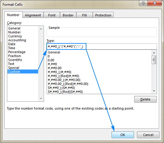
Tip. Instead of creating a custom number format from scratch, you choose a built-in Excel format close to your desired result, and customize it.
Wait, wait, but what do all those symbols in the Type box mean? And how do I put them in the right combination to display the numbers the way I want? Well, this is what the rest of this tutorial is all about 🙂
Understanding Excel number format
To be able to create a custom format in Excel, it is important that you understand how Microsoft Excel sees the number format.
An Excel number format consists of 4 sections of code, separated by semicolons, in this order:
POSITIVE; NEGATIVE; ZERO; TEXT
Here’s an example of a custom Excel format code: 
- Format for positive numbers (display 2 decimal places and a thousands separator).
- Format for negative numbers (the same as for positive numbers, but enclosed in parentheses).
- Format for zeros (display dashes instead of zeros).
- Format for text values (display text in magenta font color).
Excel formatting rules
When creating a custom number format in Excel, please remember these rules:
- A custom Excel number format changes only the visual representation, i.e. how a value is displayed in a cell. The underlying value stored in a cell is not changed.
- When you are customizing a built-in Excel format, a copy of that format is created. The original number format cannot be changed or deleted.
- Excel custom number format does not have to include all four sections.
If a custom format contains just 1 section, that format will be applied to all number types — positive, negative and zeros.
If a custom number format includes 2 sections, the first section is used for positive numbers and zeros, and the second section — for negative numbers.
A custom format is applied to text values only if it contains all four sections.
To apply the default Excel number format for any of the middle sections, type General instead of the corresponding format code.
For example, to display zeros as dashes and show all other values with the default formatting, use this format code: General; -General; «-«; General
Note. The General format included in the 2 nd section of the format code does not display the minus sign, therefore we include it in the format code.
For example, to hide zeros and negative values, use the following format code: General; ; ; General . As the result, zeros and negative value will appear only in the formula bar, but will not be visible in cells.
Digit and text placeholders
For starters, let’s learn 4 basic placeholders that you can use in your custom Excel format.
| Code | Description | Example |
| 0 | Digit placeholder that displays insignificant zeros. | #.00 — always displays 2 decimal places.
If you type 5.5 in a cell, it will display as 5.50. |
| # | Digit placeholder that only displays significant digits, without extra zeros.
That is, if a number doesn’t need a certain digit, it won’t be displayed. |
#.## — displays up to 2 decimal places.
If you type 5.5 in a cell, it will display as 5.5. If you type 5.555, it will display as 5.56. |
| ? | Digit placeholder that leaves a space for insignificant zeros on either side of the decimal point but doesn’t display them. It is often used to align numbers in a column by decimal point. | #. — displays a maximum of 3 decimal places and aligns numbers in a column by decimal point. |
| @ | Text placeholder | 0.00; -0.00; 0; [Red]@ — applies the red font color for text values. |
The following screenshot demonstrates a few number formats in action: 
As you may have noticed in the above screenshot, the digit placeholders behave in the following way:
- If a number entered in a cell has more digits to the right of the decimal point than there are placeholders in the format, the number is «rounded» to as many decimal places as there are placeholders.
For example, if you type 2.25 in a cell with #.# format, the number will display as 2.3.
All digits to the left of the decimal point are displayed regardless of the number of placeholders.
For example, if you type 202.25 in a cell with #.# format, the number will display as 202.3.
Below you will find a few more examples that will hopefully shed more light on number formatting in Excel.
| Format | Description | Input value | Display as |
| #.00 | Always display 2 decimal places. | 2 2.5 0.5556 |
2.00 2.50 .56 |
| #.## | Shows up to 2 decimal places, without insignificant zeros. | 2 2.5 0.5556 |
2. 2.5 0.56 |
| #.0# | Display a minimum of 1 and a maximum of 2 decimal places. | 2 2.205 0.555 |
2.0 2.21 .56 |
| . | Display up to 3 decimal places with aligned decimals. | 22.55 2.5 2222.5555 0.55 |
22.55 2.5 2222.556 .55 |
Excel formatting tips and guidelines
Theoretically, there are an infinite number of Excel custom number formats that you can make using a predefined set of formatting codes listed in the table below. And the following tips explain the most common and useful implementations of these format codes.
| Format Code | Description |
| General | General number format |
| # | Digit placeholder that represents optional digits and does not display extra zeros. |
| 0 | Digit placeholder that displays insignificant zeros. |
| ? | Digit placeholder that leaves a space for insignificant zeros but doesn’t display them. |
| @ | Text placeholder |
| . (period) | Decimal point |
| , (comma) | Thousands separator. A comma that follows a digit placeholder scales the number by a thousand. |
| Displays the character that follows it. | |
| » « | Display any text enclosed in double quotes. |
| % | Multiplies the numbers entered in a cell by 100 and displays the percentage sign. |
| / | Represents decimal numbers as fractions. |
| E | Scientific notation format |
| _ (underscore) | Skips the width of the next character. It’s commonly used in combination with parentheses to add left and right indents, _( and _) respectively. |
| * (asterisk) | Repeats the character that follows it until the width of the cell is filled. It’s often used in combination with the space character to change alignment. |
| [] | Create conditional formats. |
How to control the number of decimal places
The location of the decimal point in the number format code is represented by a period (.). The required number of decimal places is defined by zeros (0). For example:
- 0 or # — display the nearest integer with no decimal places.
- 0.0 or #.0 — display 1 decimal place.
- 0.00 or #.00 — display 2 decimal places, etc.
The difference between 0 and # in the integer part of the format code is as follows. If the format code has only pound signs (#) to the left of the decimal point, numbers less than 1 begin with a decimal point. For example, if you type 0.25 in a cell with #.00 format, the number will display as .25. If you use 0.00 format, the number will display as 0.25. 
How to show a thousands separator
To create an Excel custom number format with a thousands separator, include a comma (,) in the format code. For example:
- #,### — display a thousands separator and no decimal places.
- #,##0.00 — display a thousands separator and 2 decimal places.
To separate numbers with more than four digits into groups of three leaving a space between each group, use a space for the thousands separator. For example:
- # ### — rounds numbers to the nearest integer (no decimal places) separating thousands with a space.
- # ##0.00 — separate thousands with a space and display 2 decimal places.

Round numbers by thousand, million, etc.
As demonstrated in the previous tip, Microsoft Excel separates thousands by commas if a comma is enclosed by any digit placeholders — pound sign (#), question mark (?) or zero (0). If no digit placeholder follows a comma, it scales the number by thousand, two consecutive commas scale the number by million, and so on.
For example, if a cell format is #.00, and you type 5000 in that cell, the number 5.00 is displayed. For more examples, please see the screenshot below: 
Text and spacing in custom Excel number format
To display both text and numbers in a cell, do the following:
- To add a single character, precede that character with a backslash ().
- To add a text string, enclose it in double quotation marks (» «).
For example, to indicate that numbers are rounded by thousands and millions, you can add K and M to the format codes, respectively:
- To display thousands: #.00,K
- To display millions: #.00,,M
Tip. To make the number format better readable, include a space between a comma and backward slash.
The following screenshot shows the above formats and a couple more variations: 
And here is another example that demonstrates how to display text and numbers within a single cell. Supposing, you want to add the word «Increase» for positive numbers, and «Decrease» for negative numbers. All you have to do is include the text enclosed in double quotes in the appropriate section of your format code:
#.00″ Increase»; -#.00″ Decrease»; 0
Tip. To include a space between a number and text, type a space character after the opening or before the closing quote depending on whether the text precedes or follows the number, like in «Increase «. 
In addition, the following characters can be included in Excel custom format codes without the use of backslash or quotation marks:
| Symbol | Description |
| + and — | Plus and minus signs |
| ( ) | Left and right parentheses |
| : | Colon |
| ^ | Caret |
| ‘ | Apostrophe |
| Curly brackets | |
| Less-than and greater than signs | |
| = | Equal sign |
| / | Forward slash |
| ! | Exclamation point |
| & | Ampersand |
| Tilde | |
| Space character |
A custom Excel number format can also accept other special symbols such as currency, copyright, trademark, etc. These characters can be entered by typing their four-digit ANSI codes while holding down the ALT key. Here are some of the most useful ones:
| Symbol | Code | Description |
| в„ў | Alt+0153 | Trademark |
| В© | Alt+0169 | Copyright symbol |
| В° | Alt+0176 | Degree symbol |
| В± | Alt+0177 | Plus-Minus sign |
| Вµ | Alt+0181 | Micro sign |
For example, to display temperatures, you can use the format code #»В°F» or #»В°C» and the result will look similar to this: 
You can also create a custom Excel format that combines some specific text and the text typed in a cell. To do this, enter the additional text enclosed in double quotes in the 4 th section of the format code before or after the text placeholder (@), or both.
For example, to proceed the text typed in the cell with some other text, say «Shipped in«, use the following format code:
General; General; General; «Shipped in «@ 
Including currency symbols in a custom number format
To create a custom number format with the dollar sign ($), simply type it in the format code where appropriate. For example, the format $#.00 will display 5 as $5.00.
Other currency symbols are not available on most of standard keyboards. But you can enter the popular currencies in this way:
- Turn NUM LOCK on, and
- Use the numeric keypad to type the ANSI code for the currency symbol you want to display.
| Symbol | Currency | Code |
| € | Euro | ALT+0128 |
| ВЈ | British Pound | ALT+0163 |
| ВҐ | Japanese Yen | ALT+0165 |
| Вў | Cent Sign | ALT+0162 |
The resulting number formats may look something similar to this: 
If you want to create a custom Excel format with some other currency, follow these steps:
How to display leading zeros with Excel custom format
If you try entering numbers 005 or 00025 in a cell with the default General format, you would notice that Microsoft Excel removes leading zeros because the number 005 is same as 5. But sometimes, we do want 005, not 5!
The simplest solution is to apply the Text format to such cells. Alternatively, you can type an apostrophe (‘) in front of the numbers. Either way, Excel will understand that you want any cell value to be treated as a text string. As the result, when you type 005, all leading zeros will be preserved, and the number will show up as 005.
If you want all numbers in a column to contain a certain number of digits, with leading zeros if needed, then create a custom format that includes only zeros.
As you remember, in Excel number format, 0 is the placeholder that displays insignificant zeros. So, if you need numbers consisting of 6 digits, use the following format code: 000000
And now, if you type 5 in a cell, it will appear as 000005; 50 will appear as 000050, and so on: 
Tip. If you are entering phone numbers, zip codes, or social security numbers that contain leading zeros, the easiest way is to apply one of the predefined Special formats. Or, you can create the desired custom number format. For example, to properly display international seven-digit postal codes, use this format: 0000000. For social security numbers with leading zeros, apply this format: 000-00-0000.
Percentages in Excel custom number format
To display a number as a percentage of 100, include the percent sign (%) in your number format.
For example, to display percentages as integers, use this format: #%. As the result, the number 0.25 entered in a cell will appear as 25%.
To display percentages with 2 decimal places, use this format: #.00%
To display percentages with 2 decimal places and a thousands separator, use this one: #,##.00% 
Fractions in Excel number format
Fractions are special in terms that the same number can be displayed in a variety of ways. For example, 1.25 can be shown as 1 Вј or 5/5. Exactly which way Excel displays the fraction is determined by the format codes that you use.
For decimal numbers to appear as fractions, include forward slash (/) in your format code, and separate an integer part with a space. For example:
- # #/# — displays a fraction remainder with up to 1 digit.
- # ##/## — displays a fraction remainder with up to 2 digits.
- # ###/### — displays a fraction remainder with up to 3 digits.
- ###/### — displays an improper fraction (a fraction whose numerator is larger than or equal to the denominator) with up to 3 digits.
To round fractions to a specific denominator, supply it in your number format code after the slash. For example, to display decimal numbers as eighths, use the following fixed base fraction format: # #/8
The following screenshot demonstrated the above format codes in action: 
As you probably know, the predefined Excel Fraction formats align numbers by the fraction bar (/) and display the whole number at some distance from the remainder. To implement this alignment in your custom format, use the question mark placeholders (?) instead of the pound signs (#) like shown in the following screenshot: 
Tip. To enter a fraction in a cell formatted as General, preface the fraction with a zero and a space. For instance, to enter 4/8 in a cell, you type 0 4/8. If you type 4/8, Excel will assume you are entering a date, and change the cell format accordingly.
Create a custom Scientific Notation format
To display numbers in Scientific Notation format (Exponential format), include the capital letter E in your number format code. For example:
- 00E+00 — displays 1,500,500 as 1.50E+06.
- #0.0E+0 — displays 1,500,500 as 1.5E+6
- #E+# — displays 1,500,500 as 2E+6

Show negative numbers in parentheses
At the beginning of this tutorial, we discussed the 4 code sections that make up an Excel number format: Positive; Negative; Zero; Text
Most of the format codes we’ve discussed so far contained just 1 section, meaning that the custom format is applied to all number types — positive, negative and zeros.
To make a custom format for negative numbers, you’d need to include at least 2 code sections: the first will be used for positive numbers and zeros, and the second — for negative numbers.
To show negative values in parentheses, simply include them in the second section of your format code, for example: #.00; (#.00)
Tip. To line up positive and negative numbers at the decimal point, add an indent to the positive values section, e.g. 0.00_); (0.00)

Display zeroes as dashes or blanks
The built-in Excel Accounting format shows zeros as dashes. This can also be done in your custom Excel number format.
As you remember, the zero layout is determined by the 3 rd section of the format code. So, to force zeros to appear as dashes, type «-« in that section. For example: 0.00;(0.00);»-«
The above format code instructs Excel to display 2 decimal places for positive and negative numbers, enclose negative numbers in parentheses, and turn zeros into dashes.
If you don’t want any special formatting for positive and negative numbers, type General in the 1 st and 2 nd sections: General; -General; «-«
To turn zeroes into blanks, skip the third section in the format code, and only type the ending semicolon: General; -General; ; General 
Add indents with custom Excel format
If you don’t want the cell contents to ride up right against the cell border, you can indent information within a cell. To add an indent, use the underscore (_) to create a space equal to the width of the character that follows it.
The commonly used indent codes are as follows:
- To indent from the left border: _(
- To indent from the right border: _)
Most often, the right indent is included in a positive number format, so that Excel leaves space for the parentheses enclosing negative numbers.
For example, to indent positive numbers and zeros from the right and text from the left, you can use the following format code:
Or, you can add indents on both sides of the cell:
The indent codes move the data from the cell border by one character width. To move values by more than one character width, include 2 or more consecutive indent codes in your number format. The following screenshot demonstrates indenting cell contents by 1 and 2 characters: 
Change font color with custom number format
Changing the font color for a certain value type is one of the simplest things you can do with a custom number format in Excel, which supports 8 main colors. To specify the color, just type one of the following color names in an appropriate section of your number format code.
| [Black] [Green] [White] [Blue] |
[Magenta] [Yellow] [Cyan] [Red] |
Note. The color code must be the first item in the section.
For example, to leave the default General format for all value types, and change only the font color, use the format code similar to this:
Or, combine color codes with the desired number formatting, e.g. display the currency symbol, 2 decimal places, a thousands separator, and show zeros as dashes:
[Blue]$#,##0.00; [Red]-$#,##0.00; [Black]»-«; [Magenta]@ 
Repeat characters with custom format codes
To repeat a specific character in your custom Excel format so that it fills the column width, type an asterisk (*) before the character.
For example, to include enough equality signs after a number to fill the cell, use this number format: #*=
Or, you can include leading zeros by adding *0 before any number format, e.g. *0# 
This formatting technique is commonly used to change cell alignment as demonstrated in the next formatting tip.
How to change alignment in Excel with custom number format
A usual way to change alignment in Excel is using the Alignment tab on the ribbon. However, you can «hardcode» cell alignment in a custom number format if needed.
For example, to align numbers left in a cell, type an asterisk and a space after the number code, for example: «#,###* » (double quotes are used only to show that an asterisk is followed by a space, you don’t need them in a real format code).
Making a step further, you could have numbers aligned left and text entries aligned right using this custom format:
#,###* ; -#,###* ; 0* ;* @ 
This method is used in the built-in Excel Accounting format . If you apply the Accounting format to some cell, then open the Format Cells dialog, switch to the Custom category and look at the Type box, you will see this format code:
The asterisk that follows the currency sign tells Excel to repeat the subsequent space character until the width of a cell is filled. This is why the Accounting number format aligns the currency symbol to the left, number to the right, and adds as many spaces as necessary in between.
Apply custom number formats based on conditions
To have your custom Excel format applied only if a number meets a certain condition, type the condition consisting of a comparison operator and a value, and enclose it in square brackets [].
For example, to displays numbers that are less than 10 in a red font color, and numbers that are greater than or equal to 10 in a green color, use this format code:
Additionally, you can specify the desired number format, e.g. show 2 decimal places:
[Red][ =10]0.00 
And here is another extremely useful, though rarely used formatting tip. If a cell displays both numbers and text, you can make a conditional format to show a noun in a singular or plural form depending on the number. For example:
The above format code works as follows:
- If a cell value is equal to 1, it will display as «1 mile«.
- If a cell value is greater than 1, the plural form «miles» will show up. Say, the number 3.5 will display as «3.5 miles«.
Taking the example further, you can display fractions instead of decimals:
In this case, the value 3.5 will appear as «3 1/2 miles«. 
Tip. To apply more sophisticated conditions, use Excel’s Conditional Formatting feature, which is specially designed to handle the task.
Dates and times formats in Excel
Excel date and times formats are a very specific case, and they have their own format codes. For the detailed information and examples, please check out the following tutorials:
Well, this is how you can change number format in Excel and create your own formatting. Finally, here’s a couple of tips to quickly apply your custom formats to other cells and workbooks:
- A custom Excel format is stored in the workbook in which it is created and is not available in any other workbook. To use a custom format in a new workbook, you can save the current file as a template, and then use it as the basis for a new workbook.
- To apply a custom format to other cells in a click, save it as an Excel style — just select any cell with the required format, go to the Home tab >Styles group, and click New Cell Style….
To explore the formatting tips further, you can download a copy of the Excel Custom Number Format workbook we used in this tutorial. I thank you for reading and hope to see you again next week!
Источник