
To control more precisely what cells will be formatted, you can use formulas to apply conditional formatting.
Want more?
Use conditional formatting
Manage conditional formatting rule precedence
To control more precisely what cells will be formatted, you can use formulas to apply conditional formatting.
In this example, I am going to format the cells in the Product column if the corresponding cell in the In stock column is greater than 300.
I select the cells I want to conditionally format.
When you select a range of cells, the first cell you select is the active cell.
In this example, I selected from B2 through B10, so B2 is the active cell. We’ll need to know that shortly.
Create a new rule, select Use a formula to determine which cells to format. Since B2 is the active cell, I type =E2>300.
Note that in the formula, I used the relative cell reference E2 to make sure the formula adjusts to correctly format the other cells in column B.
I click the Format button and choose how I want to format the cells. I am going to use a blue fill.
Click OK to accept the color; click OK again to apply the format.
And the cells in the Product column, where the corresponding cell in column E is greater than 300, are conditionally formatted.
When I change a value in column E to greater than 300, the conditional formatting in the Product column automatically applies.
You can create multiple rules that apply to the same cells.
In this example, I want different fill colors for different ranges of scores.
I select the cells I want to apply a rule to, create a new rule that uses the rule type Use a formula to determine which cells to format.
I want to format a cell if its value is greater than or equal to 90.
The active cell is B2, so I enter the formula =B2>=90.
And configure the rule to apply a green fill when the formula is true for a cell. The cell that has a value greater than or equal to 90 is filled with green.
I create another rule for the same cells, but this time, I want to format a cell if its value is greater than or equal to 80 and less than 90.
The formula is =AND(B2>=80,B2<90).
And I choose a different fill color.
I create similar rules for 70 and 60. The last rule is for values less than 60.
The cells are now a rainbow of colors, and these are the rules we just created to enable this.
Up next, Manage conditional formatting.
In this article we will learn how to format the cells which is containing the formulas in Microsoft Excel.
To format the cells which contain formulas, we use the Conditional Formatting feature along with the ISFORMULA function in Microsoft Excel.
Conditional Formatting: —Conditional Formatting is used to highlight the important points with color in a report based on certain conditions.
ISFORMULA-This function is used to check whether a cell reference contains a formula and it returns a True or False.
For Example — We have this Excel data as shown below —
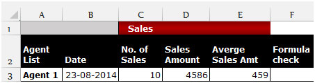
We need to check whether cell E3 containsa formula or not.
To check, follow the below given steps:-
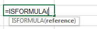
- Select the cell F3 and write the formula.
- =ISFORMULA(E3), press Enter on the keyboard.
- The function will return true.
- It means cell E3 contains a formula.
Let’s take an example to understand how we can highlight the cells which contain formulas.
We have data in range C2:G7, in which column C contains Agents name, column D contains No. of sales, column E contains sales amount and column F contains Average sales amount. We need to highlight the cells which contain the formula.
Follow the below given steps:-
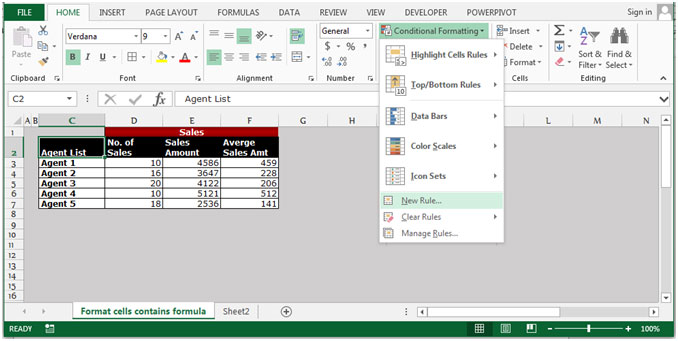
- Select the data range C3:F7.
- Go to the Home Tab.
- Select Conditional Formatting from the Styles group.
- From the Conditional formatting drop down menu, select New Rule.
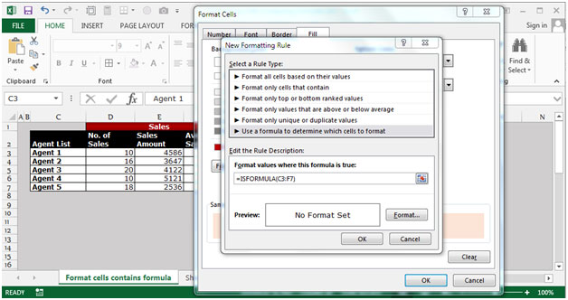
- The New Formatting Rule dialog box will appear.
- Click on “Use a formula to determine which cells to format” from Select a Rule type.
- Write the formula in Formula tab.
- =ISFORMULA(C3:F7)
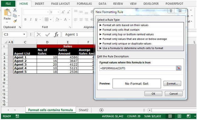
- Click on Format button.
- The Format Cells dialog box will appear.
- In the Fill tab, choose the color as per the requirement.
- Click on OK on the New Formatting Rule dialog box.
- Click on OK on the Format Cells dialog box.
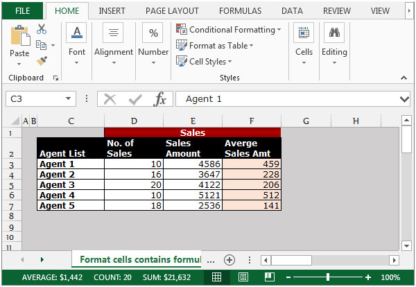
All cells which contain formulas will get highlighted with the chosen color. This is the way we can highlight the cells containing formulas in an Excel sheet by using the Conditional Formatting option along with the ISFORMULA function.
![]()
If you liked our blogs, share it with your friends on Facebook. And also you can follow us on Twitter and Facebook.
We would love to hear from you, do let us know how we can improve, complement or innovate our work and make it better for you. Write us at info@exceltip.com
I have cells with data Peer(3)
I get the number with VALUE(LEFT(RIGHT(F2,2)))
then I want to give the cell a color I am trying with but not working I get type mismatch, been trying for couple of hours and getting no where.
Thanks
Sub Format()

Dim LastRow As Long
Dim WS As Worksheet

Set WS = Sheets("sheet1")

LastRow = WS.range("F" & WS.Rows.Count).End(xlUp).Row

If WS.range("F2:F" & LastRow).Formula = "=Value(Left(Right(F2, 2)))" < 3 Then cell.Interior.ColorIndex = 10

End Sub
![]()
asked Jun 3, 2013 at 19:26
![]()
1
Perhaps
Sub Format()

Dim LastRow As Long
Dim WS As Worksheet
dim rCell as range

Set WS = Sheets("sheet1")

LastRow = WS.range("F" & WS.Rows.Count).End(xlUp).Row

for each rcell in WS.range("F2:F" & LastRow).cells
 if clng(Left(Right(rcell.value, 2), 1)) < 3 Then rcell.Interior.ColorIndex = 10
next rcell
End Sub
answered Jun 3, 2013 at 20:16
![]()
JosiePJosieP
3,3401 gold badge12 silver badges16 bronze badges
1
Instead of using VBA, use Conditional Formatting.
for e.g.
Say your cells from F1 to F10 contain values such as Peer(2), Peer(3), Peer(1) etc
- Select the Range F1 to F10 (or to any cell which you want formatted)
- On the ribbon, click on «Conditional Formatting» -> «New Rule»
- Choose «Use a formula to determine which cells to format»
- Assuming the active cell is F1, type in the formula
=VALUE(LEFT(RIGHT(F1,2))) < 3 - Click on «Format» button, go to «Fill» tab, click on «More Colors», «Custom» tab.
- Put 128 for Green, 0 for Red and Blue.
- Click «OK» till the dialog closes.
Hope that helps.
answered Jun 3, 2013 at 20:31
![]()
shahkalpeshshahkalpesh
33k3 gold badges67 silver badges88 bronze badges
2
Conditional formatting is a fantastic way to quickly visualize data in a spreadsheet. With conditional formatting, you can do things like highlight dates in the next 30 days, flag data entry problems, highlight rows that contain top customers, show duplicates, and more.
Excel ships with a large number of «presets» that make it easy to create new rules without formulas. However, you can also create rules with your own custom formulas. By using your own formula, you take over the condition that triggers a rule and can apply exactly the logic you need. Formulas give you maximum power and flexibility.
For example, using the «Equal to» preset, it’s easy to highlight cells equal to «apple».
But what if you want to highlight cells equal to «apple» or «kiwi» or «lime»? Sure, you can create a rule for each value, but that’s a lot of trouble. Instead, you can simply use one rule based on a formula with the OR function:

Here’s the result of the rule applied to the range B4:F8 in this spreadsheet:

Here’s the exact formula used:
=OR(B4="apple",B4="kiwi",B4="lime")
Quick start
You can create a formula-based conditional formatting rule in four easy steps:
1. Select the cells you want to format.

2. Create a conditional formatting rule, and select the Formula option

3. Enter a formula that returns TRUE or FALSE.

4. Set formatting options and save the rule.

The ISODD function only returns TRUE for odd numbers, triggering the rule:

Video: How to apply conditional formatting with a formula
Formula logic
Formulas that apply conditional formatting must return TRUE or FALSE, or numeric equivalents. Here are some examples:
=ISODD(A1)
=ISNUMBER(A1)
=A1>100
=AND(A1>100,B1<50)
=OR(F1="MN",F1="WI")
The above formulas all return TRUE or FALSE, so they work perfectly as a trigger for conditional formatting.
When conditional formatting is applied to a range of cells, enter cell references with respect to the first row and column in the selection (i.e. the upper-left cell). The trick to understanding how conditional formatting formulas work is to visualize the same formula being applied to each cell in the selection, with cell references updated as usual. Imagine that you entered the formula in the upper-left cell of the selection, and then copied the formula across the entire selection. If you struggle with this, see the section on Dummy Formulas below.
Formula Examples
Below are examples of custom formulas you can use to apply conditional formatting. Some of these examples can be created using Excel’s built-in presets for highlighting cells, but custom formulas can go far beyond presets, as you can see below.
Highlight orders from Texas
To highlight rows that represent orders from Texas (abbreviated TX), use a formula that locks the reference to column F:
=$F5="TX"

For more details, see this article: Highlight rows with conditional formatting.
Video: How to highlight rows with conditional formatting
Highlight dates in the next 30 days
To highlight dates occurring in the next 30 days, we need a formula that (1) makes sure dates are in the future and (2) makes sure dates are 30 days or less from today. One way to do this is to use the AND function together with the NOW function like this:
=AND(B4>NOW(),B4<=(NOW()+30))
With a current date of August 18, 2016, the conditional formatting highlights dates as follows:

The NOW function returns the current date and time. For details about how this formula, works, see this article: Highlight dates in the next N days.
Highlight column differences
Given two columns that contain similar information, you can use conditional formatting to spot subtle differences. The formula used to trigger the formatting below is:
=$B4<>$C4

See also: a version of this formula that uses the EXACT function to do a case-sensitive comparison.
Highlight missing values
To highlight values in one list that are missing from another, you can use a formula based on the COUNTIF function:
=COUNTIF(list,B5)=0

This formula simply checks each value in List A against values in the named range «list» (D5:D10). When the count is zero, the formula returns TRUE and triggers the rule, which highlights values in List A that are missing from List B.
Video: How to find missing values with COUNTIF
Highlight properties with 3+ bedrooms under $350k
To find properties in this list that have at least 3 bedrooms but are less than $300,000, you can use a formula based on the AND function:
=AND($C5<350000,$D5>=3)
The dollar signs ($) lock the reference to columns C and D, and the AND function is used to make sure both conditions are TRUE. In rows where the AND function returns TRUE, the conditional formatting is applied:

Highlight top values (dynamic example)
Although Excel has presets for «top values», this example shows how to do the same thing with a formula, and how formulas can be more flexible. By using a formula, we can make the worksheet interactive — when the value in F2 is updated, the rule instantly responds and highlights new values.

The formula used for this rule is:
=B4>=LARGE(data,input)
Where «data» is the named range B4:G11, and «input» is the named range F2. This page has details and a full explanation.
Gantt charts
Believe it or not, you can even use formulas to create simple Gantt charts with conditional formatting like this:

This worksheet uses two rules, one for the bars, and one for the weekend shading:
=AND(D$4>=$B5,D$4<=$C5) // bars
=WEEKDAY(D$4,2)>5 // weekends
This article explains the formula for bars, and this article explains the formula for weekend shading.
Simple search box
One cool trick you can do with conditional formatting is to build a simple search box. In this example, a rule highlights cells in column B that contain text typed in cell F2:

The formula used is:
=ISNUMBER(SEARCH($F$2,B2))
For more details and a full explanation, see:
- Article: How to highlight cells that contain specific text
- Article: How to highlight rows that contain specific text
- Video: How to build a search box to highlight data
Troubleshooting
If you can’t get your conditional formatting rules to fire correctly, there’s most likely a problem with your formula. First, make sure you started the formula with an equals sign (=). If you forget this step, Excel will silently convert your entire formula to text, rendering it useless. To fix, just remove the double quotes Excel added at either side and make sure the formula begins with equals (=).
If your formula is entered correctly but is not triggering the rule, you may have to dig a little deeper. Normally, you can use the F9 key to check results in a formula or use the Evaluate feature to step through a formula. Unfortunately, you can’t use these tools with conditional formatting formulas, but you can use a technique called «dummy formulas».
Dummy Formulas
Dummy formulas are a way to test your conditional formatting formulas directly on the worksheet, so you can see what they’re actually doing. This can be a big time-saver when you’re struggling to get cell references working correctly.
In a nutshell, you enter the same formula across a range of cells that matches the shape of your data. This lets you see the values returned by each formula, and it’s a great way to visualize and understand how formula-based conditional formatting works. For a detailed explanation, see this article.

Video: Test conditional formatting with dummy formulas
Limitations
There are some limitations that come with formula-based conditional formatting:
- You can’t apply icons, color scales, or data bars with a custom formula. You are limited to standard cell formatting, including number formats, font, fill color and border options.
- You can’t use certain formula constructs like unions, intersections, or array constants for conditional formatting criteria.
- You can’t reference other workbooks in a conditional formatting formula.
You can sometimes work around #2 and #3. You may be able to move the logic of the formula into a cell in the worksheet, then refer to that cell in the formula instead. If you are trying to use an array constant, try created a named range instead.
More CF formula resources
- More than 30 conditional formatting formulas examples
- Video training with practice worksheets
The best part of conditional formatting is you can use formulas in it. And, it has a very simple sense to work with formulas.
Your formula should be a logical formula and the result should be TRUE or FALSE. If the formula returns TRUE, you’ll get the formatting, and if FALSE then nothing. The point is, by using formulas you can make the best out of conditional formatting.
Yes, that’s right. In the below example, we have used a formula in CF to check whether the value in the cell is smaller than 1000 or not.

And if that value is smaller than 1000 it will apply the formatting which we have specified, otherwise not. So today in this post, I’d like to share with you simple steps to apply conditional formatting using a formula. And some of the useful examples that you can use in your daily work.
Steps to Apply Conditional Formatting with Formulas
The steps to apply CF with formulas are quite simple:
- Select the range to apply Conditional Formatting.
- Add a formula to text a condition.
- Specify a format to apply when the condition is met.

To learn this in a proper way make sure to download this sample file from here and follow the below-detailed steps.
- First of all, select the range where you want to apply conditional formatting.

- After that, go to Home Tab ➜ Styles ➜ Conditional Formatting ➜ New Rule ➜ Use a formula to determine which cell to format.

- Now, in the “Format values where formula is true” enter the below formula.
=E5<1000

- The next thing is to specify the format to apply and for this, click on the format button and select the format.

- In the end, click OK.
While entering a formula in the CF dialog box you can’t see its result or whether that formula is valid or not. So, the best practice is to check that formula before using it in CF by entering it in a cell.
1. Use a Formula that is Based on Another Cell
Yes, you can apply conditional formatting based on another cell’s value. If you look at the below example, we have added a simple formula that is based on another cell. And if the value of that linked cell meets the condition specified, you’ll get conditional formatting.

When achievement will be below 75%, it will highlight in red color.

2. Conditional Formatting using IF
Whenever I think about conditions, the first thing that comes to my mind is using the IF function. And the best part of this function is, that it fits perfectly in conditional formatting. Let me show you an example:

Here, we have used the IF to create a condition and the condition is when the count of “Done” in range B3:B9 is equal to the count of tasks in the range A3:A9, then the final status will appear.
2. Conditional Formatting with Multiple Conditions
You can create multiple checks in conditions to apply to the format. Once all the conditions or one of the conditions will meet, conditional formatting will apply to the cell. Look at the below example where we have used the average temperature of my town.
And we have used a simply combined IF-AND to highlight the months when the temperature is pretty pleasant. Months where the temperature is between 15 Celsius to 35 Celsius, will get colored.
Just like this, you can also use if with or function.
4. Highlight Alternate Rows with Conditional Formatting
To highlight every alternate row you can use the following formula n CF.
=INT(MOD(ROW(),2))
By using this formula, every row whose number is odd will be highlighted. And, if you want to do vice versa you can use the following formula.

=INT(MOD(ROW()+1,2))
The same kind of formula can use for columns (odd and even) as well.
=INT(MOD(COLUMN(),2))
And for even columns.
=INT(MOD(COLUMN()+1,2))
5. Highlight Cells with Errors using CF
Now let’s come to another example where we will check whether a cell contains an error or not. What we need to do is just insert a formula in conditional formatting that can check the condition and return the result in TRUE or FALSE. You can even verify cells for numbers, text, or some specific values as well.

6. Create a Checklist with Conditional Formatting
Now let’s add some creativity to intelligence. You have already learned how to use a formula that is based on another cell. Here we have linked a checkbox with the B1 cell and further linked the B1 with the formula used in conditional formatting for cell A1.

Now, if you tick mark the checkbox, the value of cell B1 will turn into TRUE and cell A1 gets it conditional formatting [strikethrough].
Points to Remember
- Your formula should be a logical formula, which leads to a result as TRUE or FALSE.
- Try not to overload your data with conditional formatting.
- Always use relative and absolute references in a proper sense.
Sample File
Download this sample file from here to learn more.
More Tutorials
- AUTO FORMAT Option in Excel
- Apply Accounting Number Format in Excel
- Apply Background Color to a Cell or the Entire Sheet in Excel
- Print Excel Gridlines
- Add Page Number in Excel
- Apply Comma Style in Excel
- Apply Strikethrough in Excel
- Highlight Blank Cells in Excel
- Make Negative Numbers Red in Excel
- Cell Style (Title, Calculation, Total, Headings…) in Excel
- Change Date Format in Excel
- Highlight Alternate Rows in Excel with Color Shade
- Use Icon Sets in Excel (Conditional Formatting)
- Add Border in Excel
- Change Border Color in Excel
- Clear Formatting in Excel
- Copy Formatting in Excel
- Best Fonts for Microsoft Excel
- Hide Zero Values in Excel
⇠ Back to Advanced Excel Tutorials