
Select the data series you want to format. Click the Format tab. Click Format Selection. Right-click a data series and select Format Data Series from the contextual menu.
Contents
- 1 How do I change the series of data in Excel?
- 2 How do I format multiple series in Excel?
- 3 How do I get rid of Series 1 in Excel?
- 4 How do you label a series in Excel?
- 5 What is F4 in Excel?
- 6 How do you select all series in Excel chart?
- 7 How do you graph 3 variables in Excel?
- 8 How do I remove a series from a data table in Excel?
- 9 Why does my Excel chart Say Series 1?
- 10 How do I remove data from a series label in Excel?
- 11 How do I format all data labels in Excel?
- 12 What is series name in Excel chart?
- 13 How do you edit data labels in Excel?
- 14 What is Alt F1 in Excel?
- 15 What does F11 do in Excel?
- 16 What does Ctrl Shift F3 do in Excel?
- 17 How do I format all data series?
- 18 How can you format data series in a chart?
- 19 How do you select all data series?
- 20 How do I create a 4 axis chart in Excel?
How do I change the series of data in Excel?
Right-click your chart, and then choose Select Data. In the Legend Entries (Series) box, click the series you want to change. Click Edit, make your changes, and click OK.
How do I format multiple series in Excel?
Working with Multiple Data Series in Excel
- Click Select Data button on the Design tab to open the Select Data Source dialog box.
- Select the series you want to edit, then click Edit to open the Edit Series dialog box.
- Type the new series label in the Series name: textbox, then click OK.
How do I get rid of Series 1 in Excel?
To remove a chart’s data series, click “Chart Filters” and then click “Select Data.” Select the series in the Legend Entries (Series) box, and then select “Remove.” Click “OK” to update the chart. Save this worksheet.
How do you label a series in Excel?
Rename a data series
- Right-click the chart with the data series you want to rename, and click Select Data.
- In the Select Data Source dialog box, under Legend Entries (Series), select the data series, and click Edit.
- In the Series name box, type the name you want to use.
What is F4 in Excel?
When you are typing your formula, after you type a cell reference – press the F4 key. Excel automatically makes the cell reference absolute! By continuing to press F4, Excel will cycle through all of the absolute reference possibilities.
How do you select all series in Excel chart?
Select the Layout Ribbon and then choose the Chart Elements picklist from the Current Selection Group. Then choose the series that you want. You won’t need to use this technique all the time, but it will help in certain situations so you need to add it to your Excel Tip and Trick bag.
How do you graph 3 variables in Excel?
How to graph three variables using a bar graph
- Open the spreadsheet containing your three variables.
- Highlight all the data including the headers.
- Head over to the insert tab.
- Navigate to the graphs section and choose a bar graph of your choice. Excel will automatically detect the number of variables and plot them.
How do I remove a series from a data table in Excel?
Tip: To quickly remove a data table from a chart, you can select it, and then press DELETE. You can also right-click the data table, and then click Delete. For additional options, click More Data Table Options, and then select the display option that you want.
Why does my Excel chart Say Series 1?
Note: If you create a chart without using row or column headers, Excel uses default names, starting with “Series 1.” You can learn more about how to create a chart to ensure your rows and columns are formatted properly. in the upper-right corner of the chart, and then select the Legend check box.
How do I remove data from a series label in Excel?
Do one of the following:
- On the Layout tab, in the Labels group, click Data Labels, and then click None.
- Click a data label one time to select all data labels in a data series or two times to select just one data label that you want to delete, and then press DELETE.
- Right-click a data label, and then click Delete.
How do I format all data labels in Excel?
To format data labels in Excel, choose the set of data labels to format. To do this, click the “Format” tab within the “Chart Tools” contextual tab in the Ribbon. Then select the data labels to format from the “Chart Elements” drop-down in the “Current Selection” button group.
What is series name in Excel chart?
A data series is just a group of related data representing a row or column from the worksheet.The name of the series is displayed in the “Name box” to the left of the formula bar. Excel uses a series formula or function to define a data series for a chart.
How do you edit data labels in Excel?
Edit the contents of a title or data label that is linked to data on the worksheet
- In the worksheet, click the cell that contains the title or data label text that you want to change.
- Edit the existing contents, or type the new text or value, and then press ENTER. The changes you made automatically appear on the chart.
What is Alt F1 in Excel?
Alt+F1: Creates an embedded chart of the data in the current range. Alt+Shift+F1: inserts a new worksheet. F2. F2: Edit the active cell and put the insertion point at the end of its contents. Or, if editing is turned off for the cell, move the insertion point into the formula bar.
What does F11 do in Excel?
F11 Creates a chart of the data in the current range in a separate Chart sheet. Shift+F11 inserts a new worksheet. Alt+F11 opens the Microsoft Visual Basic For Applications Editor, in which you can create a macro by using Visual Basic for Applications (VBA).
What does Ctrl Shift F3 do in Excel?
Ctrl + Shift + F3
This will open the Create Names from Selection window & are used to create names from row or column labels. You can create names for the selected cells from 4 options i.e. from Top row, Left column, Bottom row or Right column.
How do I format all data series?
Unfortunately you cannot select all the lines at once and format them. The only option is to format the lines individually or right click on Chart, Select data, and edit in the ‘Select Data Source’.
How can you format data series in a chart?
Select the chart element (for example, data series, axes, or titles), right-click it, and click Format . The Format pane appears with options that are tailored for the selected chart element.
How do you select all data series?
For example, if you wanted to select every label in a series, then left-click on one of the labels and press CTRL+A. All of the labels in that series will be highlighted. As a bonus, you can continue pressing CTRL+A to select all of the labels in all series, and CTRL+A again to select all labels in the chart.
How do I create a 4 axis chart in Excel?
How to Create a 4 Axis Chart in Excel
- Create a new spreadsheet in Excel.
- Type the label names of your axes in each column, for example, Axis 01, Axis 02, Axis 03, and Axis 04 as headers in columns A, B, C, and D respectively.
- Type the corresponding data for each column and row.
You can change the format of individual chart elements, such as the chart area, plot area, data series, axes, titles, data labels, or legend.
Two sets of tools are available for formatting chart elements: the Format task pane and the Chart Tools Ribbon. For the most control, use the options in the Format task pane.
Format your chart using the Format task pane
Select the chart element (for example, data series, axes, or titles), right-click it, and click Format <chart element>. The Format pane appears with options that are tailored for the selected chart element.
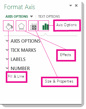
Clicking the small icons at the top of the pane moves you to other parts of the pane with more options. If you click on a different chart element, you’ll see that the task pane automatically updates to the new chart element.
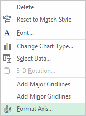
For example, to format an axis:
-
Right-click the chart axis, and click Format Axis.

-
In the Format Axis task pane, make the changes you want.
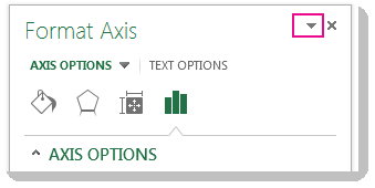
You can move or resize the task pane to make working with it easier. Click the chevron in the upper right.
-
Select Move and then drag the pane to a new location.
-
Select Size and drag the edge of the pane to resize it.
-
Format your chart using the Ribbon
-
In your chart, click to select the chart element that you want to format.
-
On the Format tab under Chart Tools, do one of the following:
-
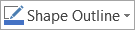
Click Shape Fill to apply a different fill color, or a gradient, picture, or texture to the chart element.
-
Click Shape Outline to change the color, weight, or style of the chart element.
-
Click Shape Effects to apply special visual effects to the chart element, such as shadows, bevels, or 3-D rotation.
-
To apply a predefined shape style, on the Format tab, in the Shape Styles group, click the style that you want. To see all available shape styles, click the More button
.
-
To change the format of chart text, select the text, and then choose an option on the mini toolbar that appears. Or, on the Home tab, in the Font group, select the formatting that you want to use.
-
To use WordArt styles to format text, select the text, and then on the Format tab in the WordArt Styles group, choose a WordArt style to apply. To see all available styles, click the More button
.
-

 .
.
You can use the Format <Chart Element> dialog box to make formatting changes, or you can apply predefined or custom shape styles. You can also format the text in a chart element.
What do you want to do?
-
Change the format of a selected chart element
-
Change the shape style of a selected chart element
-
Change the format of text in a selected chart element
-
Use text formatting to format text in chart elements
-
Use WordArt styles to format text in chart elements
Change the format of a selected chart element
-
In a chart, click the chart element that you want to change, or do the following to select the chart element from a list of chart elements:
-
Click anywhere in the chart.
This displays the Chart Tools, adding the Design, Layout, and Format tabs. -
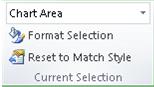
On the Format tab, in the Current Selection group, click the arrow next to the Chart Elements box, and then select the chart element that you want to format.
Tip: Instead of using the ribbon commands, you can also right-click a chart element, click Format <Chart Element> on the shortcut menu, and then continue with step 3.
-
-
On the Format tab, in the Current Selection group, click Format Selection.
-
In the Format <Chart Element> dialog box, click a category, and then select the formatting options that you want.
Important: Depending on the selected chart element, different formatting options are available in this dialog box.
-
When you select different options in this dialog box, the changes are instantly applied to the selected chart element. However, because the changes are instantly applied, it is not possible to click Cancel in this dialog box. To remove changes, you must click Undo on the Quick Access Toolbar.
-
You can undo multiple changes that you made to one dialog box option as long as you did not make changes to another dialog box option in between.
-
You may want to move the dialog box so that you can see both the chart and the dialog box at the same time.
Top of Page
Change the shape style of a selected chart element
In a chart, click the chart element that you want to change, or do the following to select the chart element from a list of chart elements:
-
Click anywhere in the chart.
This displays the Chart Tools, adding the Design, Layout, and Format tabs. -
On the Format tab, in the Current Selection group, click the arrow next to the Chart Elements box, and then select the chart element that you want to format.
To apply a predefined shape style, on the Format tab, in the Shape Styles group, click the style that you want.
Tip: To see all available shape styles, click the More button  .
.
To apply a different shape fill, click Shape Fill, and then do one of the following:
-
To use a different fill color, under Theme Colors or Standard Colors, click the color that you want to use.
Tip: Before you apply a different color, you can quickly preview how that color affects the chart. When you point to colors that you may want to use, the selected chart element will be displayed in that color on the chart.
-
To remove the color from the selected chart element, click No Fill.
-
To use a fill color that is not available under Theme Colors or Standard Colors, click More Fill Colors. In the Colors dialog box, specify the color that you want to use on the Standard or Custom tab, and then click OK.
Custom fill colors that you create are added under Recent Colors so that you can use them again. -
To fill the shape with a picture, click Picture. In the Insert Picture dialog box, click the picture that you want to use, and then click Insert.
-
To use a gradient effect for the selected fill color, click Gradient, and then under Variations, click the gradient style that you want to use.
For additional gradient styles, click More Gradients, and then in the Fill category, click the gradient options that you want to use. -
To use a texture fill, click Texture, and then click the texture that you want to use.
To apply a different shape outline, click Shape Outline, and then do one of the following:
-
To use a different outline color, under Theme Colors or Standard Colors, click the color that you want to use.
-
To remove the outline color from the selected chart element, click No Outline.
Note: If the selected element is a line, the line will no longer be visible on the chart.
-
To use an outline color that is not available under Theme Colors or Standard Colors, click More Outline Colors. In the Colors dialog box, specify the color that you want to use on the Standard or Custom tab, and then click OK.
Custom outline colors that you create are added under Recent Colors so that you can use them again. -
To change the weight of a line or border, click Weight, and then click the line weight that you want to use.
For additional line style or border style options, click More Lines, and then click the line style or border style options that you want to use. -
To use a dashed line or border, click Dashes, and then click the dash type that you want to use.
For additional dash-type options, click More Lines, and then click the dash type that you want to use. -
To add arrows to lines, click Arrows, and then click the arrow style that you want to use. You cannot use arrow styles for borders.
For additional arrow style or border style options, click More Arrows, and then click the arrow setting that you want to use.
To apply a different shape effect, click Shape Effects, click an available effect, and then select the type of effect that you want to use.
Note: Available shape effects depend on the chart element that you selected. Preset, reflection, and bevel effects are not available for all chart elements.
Top of Page
Change the format of text in a selected chart element
To format the text in chart elements, you can use regular text formatting options, or you can apply a WordArt format.
Use text formatting to format text in chart elements
-
Click the chart element that contains the text that you want to format.
-
Right-click the text or select the text that you want to format, and then do one of the following:
-
Click the formatting options that you want on the Mini toolbar.
-
On the Home tab, in the Font group, click the formatting buttons that you want to use.
-
Top of Page
Use WordArt styles to format text in chart elements
-
In a chart, click the chart element that contains the text that you want to change, or do the following to select the chart element from a list of chart elements:
-
Click anywhere in the chart.
This displays the Chart Tools, adding the Design, Layout, and Format tabs. -
On the Format tab, in the Current Selection group, click the arrow next to the Chart Elements box, and then select the chart element that you want to format.
-
-
On the Format tab, in the WordArt Styles group, do one of the following:
-
To apply a predefined WordArt style, click the style that you want.
Tip: To see all available WordArt styles, click the More button
. -
To apply a custom WordArt style, click Text Fill, Text Outline, or Text Effects, and then select the formatting options that you want.
-
Top of Page
Need more help?
You can always ask an expert in the Excel Tech Community or get support in the Answers community.

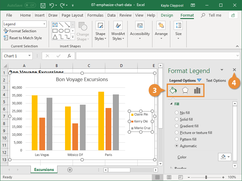
How to Format Chart Data in Excel
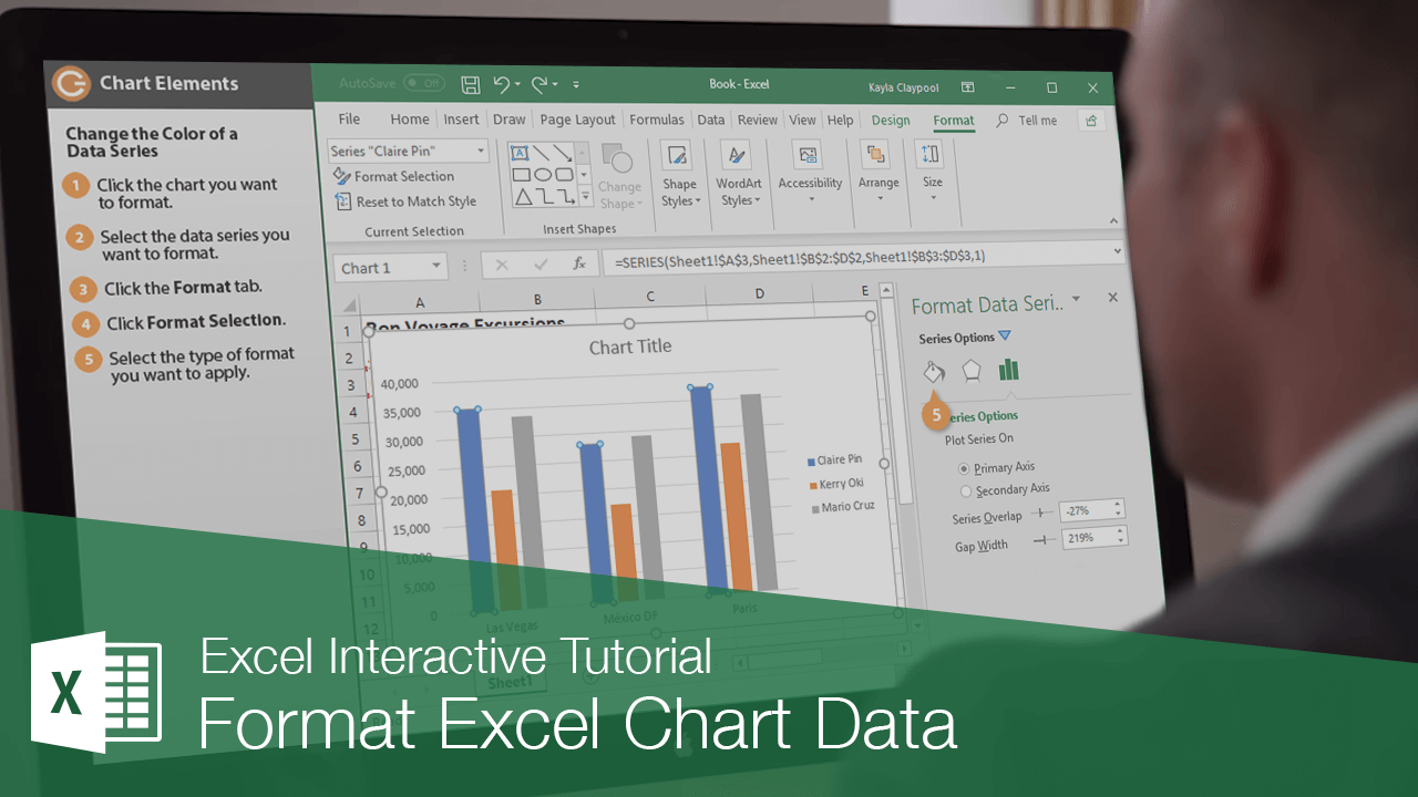
One way to emphasize chart data is to change the formatting of a specific piece of data or a data series so it stands out from the rest of the chart.
Change the Color of a Data Series
You can make a data series stand out by applying a different color to the series.
- Select the chart you want to format.
- Select the data series you want to format.
- Click the Format tab.
- Click Format Selection.

Right-click a data series and select Format Data Series from the contextual menu.
The formatting pane appears at the right.
- Click the Fill & Line button.
- Click Fill to expand the section.
- Click the Fill Color button.
- Select a color.
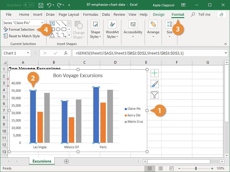
The formatting is applied to the entire data series.
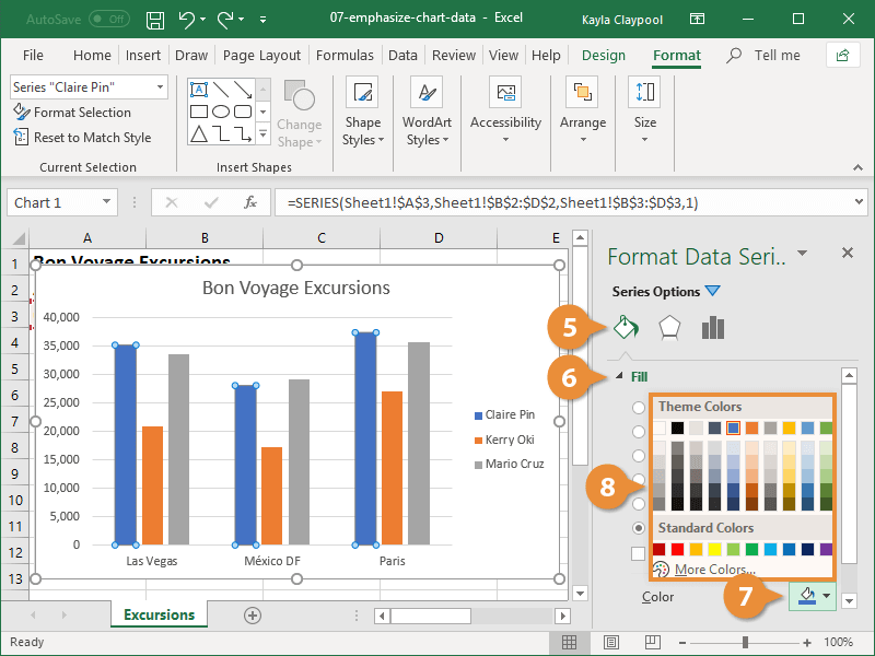
Format Other Chart Areas
You can also switch the chart element you want to format from right within the formatting panel.
- Click the Series Options menu arrow.
- Select a chart area to format.
- Select a type of format you want to apply.
- Close the Format pane.

FREE Quick Reference
Click to Download
Free to distribute with our compliments; we hope you will consider our paid training.
Tuesday, September 24, 2019
Peltier Technical Services, Inc., Copyright © 2023, All rights reserved.
Data in an Excel chart is governed by the SERIES formula. This formula is only valid in a chart, not in any worksheet cell, but it can be edited just like any other Excel formula.
Select a series in a chart. The source data for that series, if it comes from the same worksheet, is highlighted in the worksheet. And a formula appears in the Formula Bar.
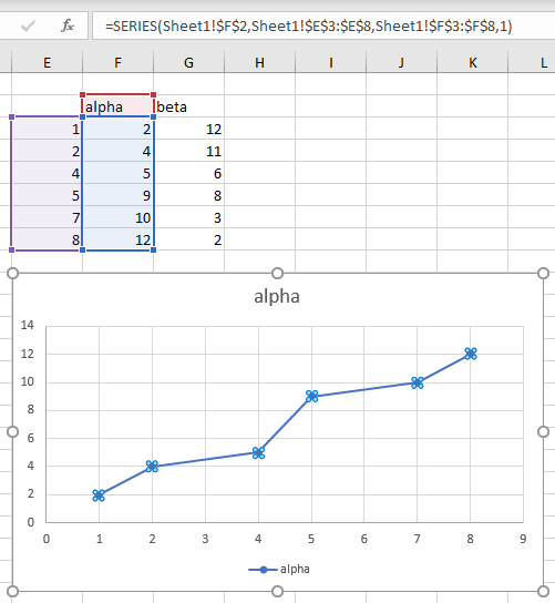
You didn’t have to write the formula. Excel writes it for you when you create a chart or added a series.
The formula in the chart shown above is:
=SERIES(Sheet1!$F$2,Sheet1!$E$3:$E$8,Sheet1!$F$3:$F$8,1)The arguments are identified as follows:
=SERIES(<series name>,<x values>,<y values>,<plot order>)In the case of a bubble chart, there is one additional argument:
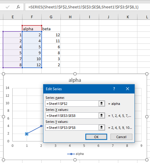
=SERIES(<series name>,<x values>,<y values>,<plot order>,<bubble size>)You can also view the series data using the Select Data dialog. Right click on the chart and choose Select Data, then select the series in the list and click the Edit button. The Edit Series dialog shows the same data that the SERIES formula shows.
Here are a few valid SERIES formulas. This formula has conventional cell addresses:
=SERIES(Sheet1!$F$2,Sheet1!$E$3:$E$8,Sheet1!$F$3:$F$8,1)This formula plots the same, although the values are not linked to the worksheet, but are instead hard-coded into the formula:
=SERIES("alpha",{1,2,4,5,7,8},{2,4,5,9,10,12},1)This formula doesn’t even include a Series Name or Y Values, and the Y Values are represented by a Name (Named Range).
=SERIES(,,SERIESFormula!YValues,1)Series Formula Arguments
Series Name
Series Name is obviously the name of the series, and it’s what is displayed in a legend. This argument is usually a cell reference, Sheet1!$F$2, but it can also be a hard-coded string enclosed in double quotes, "alpha", or it can be left blank. If it is blank, the series name will be “Series N“, where N is the number of the series.
X Values
X Values are the numbers or category labels plotted along the X axis (category axis) of the chart, usually the horizontal axis but the vertical axis of a horizontal bar chart. This is usually a cell reference, Sheet1!$E$3:$E$8, but it can also be a hard-coded array in curly braces, {1,2,4,5,7,8} or {"A","B","C","D","E","F"}, and it can be left blank. If x Values is left blank, the series will either use the same X values as the first series in the chart uses, or it uses the counting numbers {1,2,3,etc.}. Note that in non XY Scatter charts, all series use the same X values as the first series in the chart.
Y Values
Y Values are the numbers plotted along the Y axis (value axis) of the chart, usually the vertical axis but the horizontal axis of a horizontal bar chart. This is usually a cell reference, Sheet1!$F$3:$F$8, but it can also be a hard-coded array in curly braces, {2,4,5,9,10,12}. Y values cannot be left blank; if you try, Excel will remind you that a series must contain at least one value. A text value in the Y Values will be plotted as a zero.

Plot Order
Plot Order is a series number within the chart. This is always a number between 1 and the number of series in the chart.
“Plot Order” is a bit of a misnomer, because regardless of this number, some types of series are plotted before others. For example, all area series are plotted before all bar/column series, and those are plotted before line series, and XY scatter series are plotted last of all. Within each chart group, all primary series are plotted before all secondary series. So “Series Number” would be a better name.
Bubble Size
Bubble Size contains the numbers used to calculate the diameters of the bubbles in a bubble chart. This is usually a cell reference, Sheet1!$G$3:$G$8, but it can also be a hard-coded array in curly braces, {12,11,6,8,3,2}. I’ve noticed that the first element in a hard-coded array is ignored, so I pad it at the beginning with a dummy bubble size of zero: {0,12,11,6,8,3,2}. Bubble Sizes cannot be left blank; if you try, Excel will remind you that a series must contain at least one value (using the same message as for blank Y Values.
Editing SERIES Formulas
Just like any formula in Excel, you can edit the series formula right in the Formula Bar, and the new formula will change the output.
While it’s pretty easy to modify a series’ data by dragging the highlighted regions in the worksheet, you can just as easily change “F” in this series formula
=SERIES(Sheet1!$F$2,Sheet1!$E$3:$E$8,Sheet1!$F$3:$F$8,1)to “G”, and the chart will use the series name and Y values in column G.
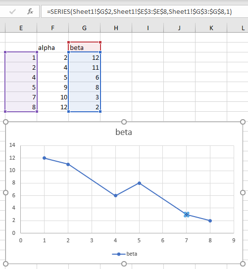
And both of these techniques are easier than going through the whole Select Data > Edit Series routine.
You can modify any of the arguments. You can change the series name, the X and Y values, and even the series number (plot order). You can type right in the formula, and you can use the mouse to select ranges. Just be careful not to break syntax.
You can also add a new series to a chart by entering a new SERIES formula. Select the chart area of a chart, click in the Formula Bar (or not, Excel will assume you’re typing a SERIES formula), and start typing. It’s even quicker if you copy another series formula, select the chart area, click in the formula bar, paste, and edit.
Cell References and Arrays in the SERIES Formula
Normal Cell References
If you are referencing a cell address, you need to qualify the address with the worksheet name, Sheet1!$F$2. If you try to enter an unqualified reference, $F$2, Excel will give you a warning:
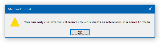
The SERIES formula always uses absolute references, Sheet1!$F$2 as opposed to Sheet1!F2. If you enter a relative reference, Sheet1!F2, Excel will automatically convert it to an absolute reference without any hassle.
Fragmented Ranges
The ranges used for X or Y Values do not need to be contiguous. The following formula is perfectly valid. Both the X Values and Y Values consist of ranges with two areas, with the two areas enclosed in parentheses.
=SERIES(Sheet1!$F$2,(Sheet1!$E$3:$E$5,Sheet1!$E$7:$E$9),(Sheet1!$F$3:$F$5,Sheet1!$F$7:$F$9),1)I made use of this trick in Add One Trendline for Multiple Series, where I build an uber-formula containing data from all series in a chart (such as the formula below, for three series), and add a trendline that fits all of this data.
=SERIES("Combined",(Sheet1!$B$3:$B$11,Sheet1!$D$3:$D$11,Sheet1!$F$3:$F$11),
(Sheet1!$C$3:$C$11,Sheet1!$E$3:$E$11,Sheet1!$G$3:$G$11),4)
Ranges in Other Workbooks
A chart can reference ranges in external workbooks, as long as the ranges are properly references by workbook and worksheet.
=SERIES([SERIESFormula.xlsm]Sheet1!$F$2,[SERIESFormula.xlsm]Sheet1!$E$3:$E$8,[SERIESFormula.xlsm]Sheet1!$F$3:$F$8,1)Names (Named Ranges)
If your references are Names (Named Ranges), you need to qualify the Name with the scope of the Name, that is, either its parent worksheet or the parent workbook.
=SERIES(Sheet1!TheSeriesName,Sheet1!TheXValues,Sheet1!TheYValues,1)You can enter the Name qualified by the worksheet, and if the Name is scoped to the workbook, Excel will fix it for you.
=SERIES(SERIESFormula.xlsm!TheSeriesName,SERIESFormula.xlsm!TheXValues,SERIESFormula.xlsm!TheYValues,1)Note that the Names you use in a SERIES formula cannot begin with the letters C or R (upper or lower case). You can still use these Names, but you need to use the Select Data Source/Edit Series dialogs to add them.
Arrays
When you use a hard-coded array in a SERIES formula, text values must each be surrounded by double quotes, {“D”,”E”,”F”}, while numerical values should not, {4,5,6}. If numbers are surrounded with quotes, {“4″,”5″,”6”}, they will be treated as text labels in the X Values. In an XY scatter chart, they won’t even appear in the chart, but Excel will use counting numbers {1,2,3} for X Values and zero for Y Values.
Using VBA with the SERIES Formula
Knowing how the SERIES formula works, and having a small bit of knowledge VBA, there is no shortage of charting features you can build with VBA.
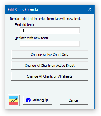
Edit SERIES Formulas (Find-Replace)
There is no built-in Find-and-Replace feature that works with SERIES formulas, but I’ve built my own. It’s based loosely on the following with a lot of error checking that I’ve had to add.
But it’s handy for changing a sheet name (e.g., Sheet1 to Sheet2) or column or row (column $A$ to B or row $5 to 10). Note that I use absolute partial references for columns and rows. Otherwise, I might want to change column S to column Q, and I’d change SERIES to QERIEQ, which would just break.
The following simple macro asks the user for two strings, one to find, and one to change to, and it changes all series in the active chart.
Sub ChangeSeriesFormula_ActiveChart()
  ''' Just do active chart
  If ActiveChart Is Nothing Then
    '' There is no active chart
    MsgBox "Please select a chart and try again.", vbExclamation, _
      "No Chart Selected"
    Exit Sub
  End If

  Dim OldString As String
  OldString = InputBox("Enter the string to be replaced:", "Enter old string")

  If Len(OldString) > 1 Then
    Dim NewString As String
    NewString = InputBox("Enter the string to replace " & """" _
      & OldString & """:", "Enter new string")
    '' Loop through all series
    Dim srs As Series
    For Each srs In ActiveChart.SeriesCollection
      Dim NewFormula As String
      NewFormula = WorksheetFunction.Substitute(mySrs.Formula, _
        OldString, NewString)
      srs.Formula = strTemp
    Next
  Else
    MsgBox "Nothing to be replaced.", vbInformation, "Nothing Entered"
  End If
End Sub
See How To: Use Someone Else’s Macro if you’re not sure how to implement this, or leave a comment below (I check frequently), or shoot me an email. You can modify it to work on all charts on the active sheet, or whatever you like.
This simple code, with about ten times as many lines devoted to checking for user errors and the many eccentricities of Excel, forms the basis of a popular feature in Peltier Tech Charts for Excel.
More VBA & SERIES Formula Examples
I have many more examples of VBA that uses SERIES formulas to get a certain result.
Add Names to Chart Series
Sometimes you are in a hurry to make a chart, and you don’t include the range with the series names. In Simple VBA Code to Manipulate the SERIES Formula and Add Names to Excel Chart Series I have code that determines how the data is plotted, and picks the cell above a column of Y values or to the left of a row of Y values for the name of each series in a chart.
Add Series to Existing Chart
In Add Series to Existing Chart I use VBA to find the last series in a chart, and add another series using the next row or column of data.
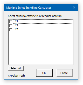
Multiple Trendline Calculator
Trendline Calculator for Multiple Series shows code that combines data from multiple series into one big series, and generates a single trendline from this larger series.
Switch X and Y Values (or Axes)
In Switch X and Y Values in a Scatter Chart, I show how to switch the X and Y components of the SERIES formula to switch the X and Y axes of a scatter chart. This is the basis of another feature in Peltier Tech Charts for Excel.

Peltier Tech Consulting Services
I enjoy doing this kind of project. Even with the ribbon components and the dialog, it only takes a few hours. And a few hours of my work will save you time every time you use the result. If you need something like this, send me your requirements and I’ll generate a quote.
Coming to You From…
Sometimes it’s easier to get into blogging from someplace that’s not my office. I used to go to a coffee shop, but that’s so cliché, and it actually doesn’t even work anymore. So today I’m writing from the newest craft brewery in Worcester, Redemption Rock. Maybe I can write it off as a business lunch!

I sampled two very nice IPAs, one very hazy, and two fine stouts, one a nitro stout that was very nice. And they have a nice concoction that combines cold-brewed coffee with the nitro stout, mmmmm.
In Excel, there is 3 different ways to create your series of number or date
- The fill-handle
- The fill menu
- SEQUENCE function
Fill series of numbers
If you want to create a series of numbers quickly, the trick is simple
- Write the first value
- Write the second value
- Select the 2 cells
- Use the fill handle to extend the selection

Excel will extend the selection according to the step between the 2 numbers.
Look at this video to see how it works with positives, negatives, and decimal numbers.
Fill series for thousands of data
But if you have to create an extensive list of numbers, using the fill handle is useless because it takes too much time 😤
It’s better to use the tool Home > Fill > Series

In the dialog box, you fill these parameters
- Select the cell containing the starting value
- Select the orientation (here columns because you want the result in the same column)
- Indicate the step (by default it’s 1)
- Indicate the last value to reach

And the result is a list of values starting from 1 to 5000 with a step of 2 😀👍

Fill a series with SEQUENCE
If you work with Excel 365, Excel Online, or Excel 2021, you can use the SEQUENCE function to create your series of number
=SEQUENCE(number of rows, number of columns, starting value, step)
For instance, to create a series from 0 to 50 with a step of 5, you write the following formula
=SEQUENCE(10, ,0,5)

Then, to convert the result of your formula to value, you must perform a copy-paste value
Create a series of dates
If you want to create a series of dates, the 3 same techniques (fill handle, tool Fill series, and SEQUENCE) can be used. But also Excel respects the number of days in a month.
For example, you can easily create a series of weeks with a step of 7 days

And the same technique can be used with the months.
- You write the 2 first months
- You select the 2 cells
- Expand the selection
