
Data entry can sometimes be a big part of using Excel.
With near endless cells, it can be hard for the person inputting data to know where to put what data.
A data entry form can solve this problem and help guide the user to input the correct data in the correct place.
Excel has had VBA user forms for a long time, but they are complicated to set up and not very flexible to change.
In this blog post, we’re going to explore 5 easy ways to create a data entry form for Excel.
Video Tutorial
Excel Tables
We’ve had Excel tables since Excel 2007.
They’re perfect data containers and can be used as a simple data entry form.
Creating a table is easy.
- Select the range of data including the column headings.
- Go to the Insert tab in the ribbon.
- Press the Table button in the Tables section.
We can also use a keyboard shortcut to create a table. The Ctrl + T keyboard shortcut will do the same thing.
Make sure the Create Table dialog box has the My table has headers option checked and press the OK button.
We now have our data inside an Excel table and we can use this to enter new data.
To add new data into our table we can start typing a new entry into the cells directly below the table and the table will absorb the new data.
We can use the Tab key instead of Enter while entering our data. This will cause the active cell cursor to move to the right instead of down so we can add the next value into our record.
When the active cell cursor is in the last cell of the table (lower right cell), pressing the Tab key will create a new empty row in the table ready for the next entry.
This is a perfect and simple data entry form.
Data Entry Form
Excel actually has a hidden data entry form and we can access it by adding the command to the Quick Access Toolbar.
Add the form command to the Quick Access Toolbar.
- Right click anywhere on the quick quick access toolbar.
- Select Customize Quick Access Toolbar from the menu options.
This will open up the Excel option menu on the Quick Access Toolbar tab.
- Select Commands Not in the Ribbon.
- Select Form from the list of available commands. Press F to jump to the commands starting with F.
- Press the Add button to add the command into the quick access toolbar.
- Press the OK button.
We can then open up data entry form for any set of data.
- Select a cell inside the data which we want to create a data entry form with.
- Click on the Form icon in the quick access toolbar area.
This will open up a customized data entry form based on the fields in our data.
Microsoft Forms
If we need a simple data entry form, why not use Microsoft Forms?
This form option will require our Excel workbook to be saved into SharePoint or OneDrive.
The form will be in a browser and not in Excel, but we can link the form to an Excel workbook so that all the data goes into our Excel table.
This is a great option if multiple people or people outside our organization need to input data into the Excel workbook.
We need to create a Form for Excel in either SharePoint or OneDrive. The process is the same for both SharePoint or OneDrive.
- Go to a SharePoint document library or a OneDrive folder where the Excel workbook is going to be saved.
- Click on New and then choose Forms for Excel.
This will prompt us to name the Excel workbook and open up a new browser tab where we can build our form by adding different types of questions.
We first need to create the Form and this will create the table in our Excel workbook where the data will get populated.
Then we can share the form with anyone we want to input data into Excel.
When a user enters data into the form and presses the submit button, that data will automatically show up into our Excel workbook.
Power Apps
Power Apps is a flexible drag and drop formula based app building platform from Microsoft.
We can certainly use it to create a data entry from for our Excel data.
In fact, if we have a table of data set up, Power Apps will create the app for us based on our data. It can’t be any easier than that.
Sign in to the powerapps.microsoft.com service ➜ go to the Create tab in the navigation pane ➜ select Excel Online.
We’ll then be prompted to sign in to our SharePoint or OneDrive account where our Excel file is saved to select the Excel workbook and table with our data.
This will generate us a fully functional three screen data entry app.
- We can search and view all the records in our Excel table in a scroll-able gallery.
- We can view an individual record in our data.
- We can edit an existing record or add new records.
This is all connected to our Excel table, so any changes or additions from the app will show up in Excel.
Power Automate
Power Automate is a cloud based tool for automating task between apps.
But we can use the button trigger to make an automation that captures user input and adds the data into an Excel table.
We’ll need to have our Excel workbook saved in OneDrive or SharePoint and have a table already setup with the fields we want to populate.
To create our Power Automate data entry form.
- Go to flow.microsoft.com and sign in.
- Go to the Create tab.
- Create an Instant flow.
- Give the flow a name.
- Choose the Manually trigger a flow option as the trigger.
- Press the Create button.
This will open up the Power Automate builder and we can build our automation.
- Click on the Manually trigger a flow block to expand the trigger’s options. This is where we’ll find the ability to add input fields.
- Click on the Add an input button. This will give us options to add a few different types of input fields including Text, Yes/No, Files, Email, Number and Dates.
- Rename the field to something descriptive. This will help the user know what type of data to input when they run this automation.
- Click on the three ellipses to the right of each field to change the input options. We’ll be able to Add a drop-down list of option, Add a multi-select list of options, Make the field optional or Delete the field from this menu.
- After we have added all our input fields, we can now add a New step to the automation.
Search for the Excel connector and add the Add a row into a table action. If you’re on an Office 365 business account, use the Excel Online (Business) connectors, otherwise use the Excel Online (OneDrive) connectors.
Now we can set up our Excel Add a row into a table step.
- Navigate to the Excel file and table where we are going to be adding data.
- After selecting the table, the fields in that table will appear listed and we can add the appropriate dynamic content from the Manually trigger a flow trigger step.
Now we can run our Flow from the Power Automate service.
- Go to My flows in the left navigation pane.
- Go to the My flows tab.
- Find the flow in the list of available flows and click on the Run button.
- A side pane will pop up with our inputs and we can enter our data.
- Click Run flow.
We can also run this from our mobile device with the Power Automate apps.
- Go to the Buttons section in the app.
- Press on the flow to run.
- Enter the data inputs in the form.
- Press on the DONE button in the top right.
Whichever way we run the flow, a few seconds later the data will appear in our Excel table.
Conclusions
Whether we require a simple form or something more complex and customize-able, there is a solution for our data entry needs.
We can quickly create something inside our workbook or use an external solution that connects to and loads data into Excel.
We can even create forms that people outside our organization can use to populate our spreadsheets.
Let me know in the comments what is your favourite data entry form option.
About the Author
John is a Microsoft MVP and qualified actuary with over 15 years of experience. He has worked in a variety of industries, including insurance, ad tech, and most recently Power Platform consulting. He is a keen problem solver and has a passion for using technology to make businesses more efficient.
Watch the Video on Using Data Entry Forms in Excel
Below is a detailed written tutorial about Excel Data Entry form in case you prefer reading over watching a video.
Excel has many useful features when it comes to data entry.
And one such feature is the Data Entry Form.
In this tutorial, I will show you what are data entry forms and how to create and use them in Excel.
Why Do You Need to Know About Data Entry Forms?
Maybe you don’t!
But if data entry is a part of your daily work, I recommend you check out this feature and see how it can help you save time (and make you more efficient).
There are two common issues that I have faced (and seen people face) when it comes to data entry in Excel:
- It’s time-consuming. You need to enter the data in one cell, then go to the next cell and enter the data for it. Sometimes, you need to scroll up and see which column it is and what data needs to be entered. Or scroll to the right and then come back to the beginning in case there are many columns.
- It’s error-prone. If you have a huge data set which needs 40 entries, there is a possibility you may end up entering something that was not intended for that cell.
A data entry form can help by making the process faster and less error-prone.
Before I show you how to create a data entry form in Excel, let me quickly show you what it does.
Below is a data set that is typically maintained by the hiring team in an organization.
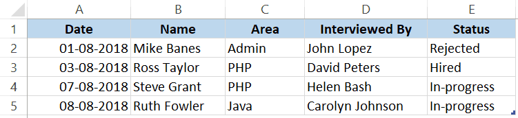
Every time a user has to add a new record, he/she will have to select the cell in the next empty row and then go cell by cell to make the entry for each column.
While this is a perfectly fine way of doing it, a more efficient way would be to use a Data Entry Form in Excel.
Below is a data entry form that you can use to make entries to this data set.
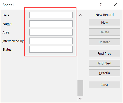
The highlighted fields are where you would enter the data. Once done, hit the Enter key to make the data a part of the table and move on to the next entry.
Below is a demo of how it works:
As you can see, this is easier than regular data entry as it has everything in a single dialog box.
Data Entry Form in Excel
Using a data entry form in Excel needs a little pre-work.
You would notice that there is no option to use a data entry form in Excel (not in any tab in the ribbon).
To use it, you will have to first add it to the Quick Access Toolbar (or the ribbon).
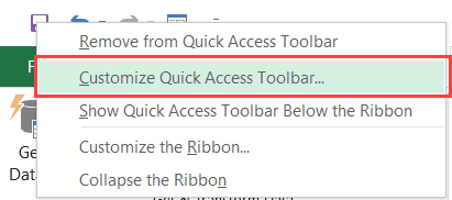
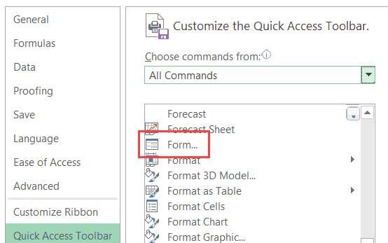
Adding Data Entry Form Option To Quick Access Toolbar
Below are the steps to add the data entry form option to the Quick Access Toolbar:
- Right-click on any of the existing icons in the Quick Access Toolbar.
- Click on ‘Customize Quick Access Toolbar’.

- In the ‘Excel Options’ dialog box that opens, select the ‘All Commands’ option from the drop-down.

- Scroll down the list of commands and select ‘Form’.

- Click on the ‘Add’ button.

- Click OK.


The above steps would add the Form icon to the Quick Access Toolbar (as shown below).
![]()
Once you have it in QAT, you can click any cell in your dataset (in which you want to make the entry) and click on the Form icon.
Note: For Data Entry Form to work, your data should be in an Excel Table. If it isn’t already, you’ll have to convert it into an Excel Table (keyboard shortcut – Control + T).
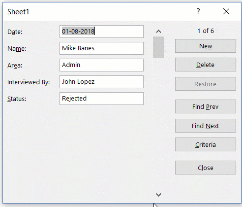
Parts of the Data Entry Form
A Data Entry Form in Excel has many different buttons (as you can see below).
Here is a brief description of what each button is about:
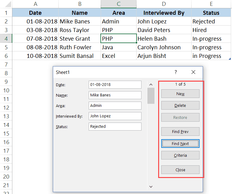
- New: This will clear any existing data in the form and allows you to create a new record.
- Delete: This will allow you to delete an existing record. For example, if I hit the Delete key in the above example, it will delete the record for Mike Banes.
- Restore: If you’re editing an existing entry, you can restore the previous data in the form (if you haven’t clicked New or hit Enter).
- Find Prev: This will find the previous entry.
- Find Next: This will find the next entry.
- Criteria: This allows you to find specific records. For example, if I am looking for all the records, where the candidate was Hired, I need to click the Criteria button, enter ‘Hired’ in the Status field and then use the find buttons. Example of this is covered later in this tutorial.
- Close: This will close the form.
- Scroll Bar: You can use the scroll bar to go through the records.
Now let’s go through all the things you can do with a Data Entry form in Excel.
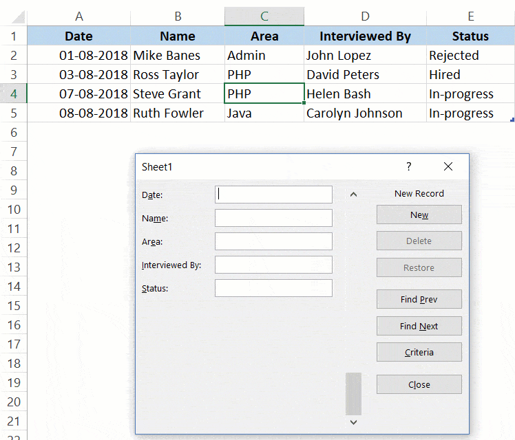
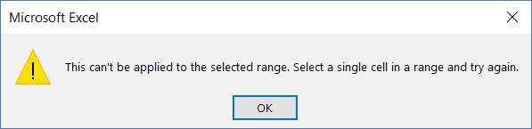
Note that you need to convert your data into an Excel Table and select any cell in the table to be able to open the Data Entry form dialog box.
If you haven’t selected a cell in the Excel Table, it will show a prompt as shown below:
Creating a New Entry
Below are the steps to create a new entry using the Data Entry Form in Excel:
- Select any cell in the Excel Table.
- Click on the Form icon in the Quick Access Toolbar.

- Enter the data in the form fields.
- Hit the Enter key (or click the New button) to enter the record in the table and get a blank form for next record.
Navigating Through Existing Records
One of the benefits of using Data Entry Form is that you can easily navigate and edit the records without ever leaving the dialog box.
This can be especially useful if you have a dataset with many columns. This can save you a lot of scrolling and the process of going back and forth.
Below are the steps to navigate and edit the records using a data entry form:
- Select any cell in the Excel Table.
- Click on the Form icon in the Quick Access Toolbar.
- To go to the next entry, click on the ‘Find Next’ button and to go to the previous entry, click the ‘Find Prev’ button.

- To edit an entry, simply make the change and hit enter. In case you want to revert to the original entry (if you haven’t hit the enter key), click the ‘Restore’ button.
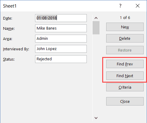
You can also use the scroll bar to navigate through entries one-by-one.
The above snapshot shows basic navigation where you are going through all the records one after the other.
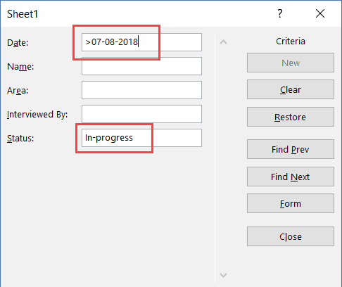
But you can also quickly navigate through all the records based on criteria.
For example, if you want to go through all the entries where the status is ‘In-progress’, you can do that using the below steps:
Criteria is a very useful feature when you have a huge dataset, and you want to quickly go through those records that meet a given set of criteria.
Note that you can use multiple criteria fields to navigate through the data.
For example, if you want to go through all the ‘In-progress’ records after 07-08-2018, you can use ‘>07-08-2018’ in the criteria for ‘Date’ field and ‘In-progress’ as the value in the status field. Now when you navigate using Find Prev/Find Next buttons, it will only show records after 07-08-2018 where the status is In-progress.
You can also use wildcard characters in criteria.
For example, if you have been inconsistent in entering the data and have used variations of a word (such as In progress, in-progress, in progress, and inprogress), then you need to use wildcard characters to get these records.
Below are the steps to do this:
- Select any cell in the Excel table.
- Click on the Form icon in the Quick Access Toolbar.
- Click the Criteria button.
- In the Status field, enter *progress
- Use the Find Prev/Find Next buttons to navigate through the entries where the status is In-Progress.

This works as an asterisk (*) is a wildcard character that can represent any number of characters in Excel. So if the status contains the ‘progress’, it will be picked up by Find Prev/Find Next buttons no matter what is before it).
Deleting a Record
You can delete records from the Data Entry form itself.
This can be useful when you want to find a specific type of records and delete these.
Below are the steps to delete a record using Data Entry Form:
- Select any cell in the Excel table.
- Click on the Form icon in the Quick Access Toolbar.
- Navigate to the record you want to delete
- Click the Delete button.

While you may feel that this all looks like a lot of work just to enter and navigate through records, it saves a lot of time if you’re working with lots of data and have to do data entry quite often.
Restricting Data Entry Based on Rules
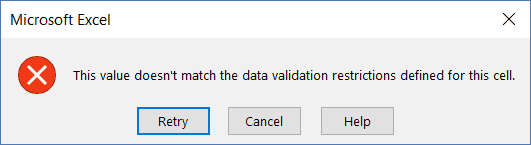
You can use data validation in cells to make sure the data entered conforms to a few rules.
For example, if you want to make sure that the date column only accepts a date during data entry, you can create a data validation rule to only allow dates.
If a user enters a data that is not a date, it will not be allowed and the user will be shown an error.
Here is how to create these rules when doing data entry:
- Select the cells (or even the entire column) where you want to create a data validation rule. In this example, I have selected column A.
- Click the Data tab.

- Click the Data Validation option.

- In the ‘Data Validation’ dialog box, within the ‘Settings’ tab, select ‘Date’ from the ‘Allow’ drop down.

- Specify the start and the end date. Entries within this date range would be valid and rest all would be denied.
- Click OK.


Now, if you use the data entry form to enter data in the Date column, and if it isn’t a date, then it will not be allowed.
You will see a message as shown below:
Similarly, you can use data validation with data entry forms to make sure users don’t end up entering the wrong data. Some examples where you can use this is numbers, text length, dates, etc.
Here are a few important things to know about Excel Data Entry Form:
- You can use wildcard characters while navigating through the records (through criteria option).
- You need to have an Excel table to be able to use the Data Entry Form. Also, you need to have a cell selected in it to use the form. There is one exception to this though. If you have a named range with the name ‘Database’, then the Excel Form will also refer to this named range, even if you have an Excel table.
- The field width in the Data Entry form is dependent on the column width of the data. If your column width is too narrow, the same would be reflected in the form.
- You can also insert bullet points in the data entry form. To do this, use the keyboard shortcut ALT + 7 or ALT + 9 from your numeric keypad. Here is a video about bullet points.
You May Also Like the Following Excel Tutorials:
- 100+ Excel Interview Questions.
- Drop Down Lists in Excel.
- Find and Remove Duplicates in Excel.
- Excel Text to Columns.
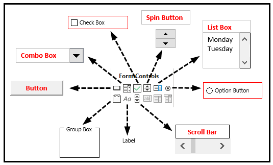
Excel Form Controls are objects that we can insert into the worksheet to work with data and handle the data as specified. For example, using these form controls in Excel, we can create a drop-down list in excelA drop-down list in excel is a pre-defined list of inputs that allows users to select an option.read more, list boxes, spinners, checkboxes, and scroll bars.
Table of contents
- Excel Form Controls
- How to use Form Controls in Excel?
- Form Control 1: Button
- Form Control 2: Combo Box
- Form Control 3: CheckBox
- Form Control 4: Spin Button
- Form Control 5: List Box
- Form Control 6: Group Box
- Form Control 7: Label
- Form Control 8: Scroll Bar
- Things to Remember
- Recommended Articles
- How to use Form Controls in Excel?
“Form Controls” is available in Excel under the “Developer” tab excel.
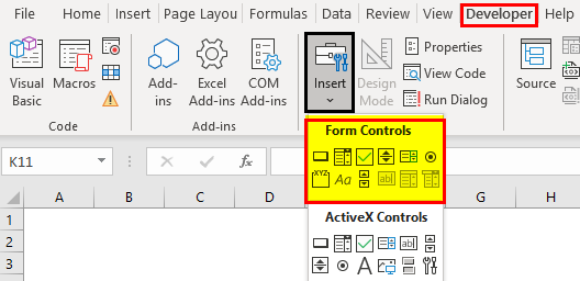
As we can see, we have two categories, “Form Controls” and “Active X Controls.” In this article, we are concentrating only on “Form Controls.” The below image describes all the “Form Controls” in Excel.
How to use Form Controls in Excel?
Now, we will see how to work with each in detail.
You can download this Form Controls Excel Template here – Form Controls Excel Template
Form Control 1: Button
This option is to draw a button and assign any macro name to it so that the assigned macro can run when we click this button.

Form Control 2: Combo Box
The combo box is our drop-down list. It works the same as the drop-down list, but combo box excelCombo Box in Excel is a type of data validation tool that can create a dropdown list for the user to select from the pre-determined list. It is a form control which is available in the insert tab of the developer’s tab.read more is considered an object.
We must select the “ComboBox” and draw anywhere on the worksheet area.

To insert values, we must create a day list in column A.

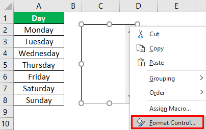
Now, select the “Combo Box,” right-click and choose “Format Control.”

Now in the “Format Control” window, choose “Control.” Then, in the “Input range,” choose the month names range of cells. Then, click on “OK.”

Now, we can see the selected day list in the combo box.

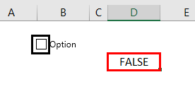
Form Control 3: CheckBox
The checkbox is used to display the item selection. If checked, we can link to a certain cell to show the selection as “TRUE” and “FALSE” if unchecked.
We must first draw the checkbox on the worksheet.

Then, right-click and choose the “Edit Text” option.

Change the default name from “Check Box1” to “Option.”

Again, right-click and choose “Format Control.”

Under the “Control” tab, we must choose “Unchecked” and give the “Cell link” to the D3 cell. Click “OK.”

Now, check the box to see the “TRUE” value in cell D3.

And uncheck the box to see the “FALSE” value.
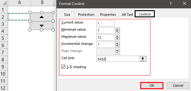
Form Control 4: Spin Button
Using the “Spin Button,” we can increment and decrement the value in the linked cell. We need to draw the spin button to see options.

Then, right-click on the button and choose “Format Control.”

Under the “Control” tab, we can make all the settings. We can set a minimum value, maximum value, and current value. Also, we can configure what should be the incremental and decremented value when the spin button is clicked. Click “OK.”
Now, if we click up the arrow of the spin button in cell A2 one, we can see the incremental value.
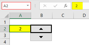
And if we click on the down arrow of a spin button in cell A2, we can see every time it will be decreased by one.

Another thing is in the “Format Control” window, we have set 1 as the “Minimum value” and 12 as the “Maximum value.”

So, when we press the up arrow, it will increment by 1 until it reaches 12. After that, it will not increase.

Form Control 5: List Box
Using the list box in excelThe list box in Excel VBA is a list assigned to a variable with a variety of inputs to select from. It allows multiple options to be selected at the same time and can be added on a UserForm using the list box option.read more, we can create a list of items. Let’s first draw the box and then configure it.

For this list box, we will create a list of days.

Then, right-click on the “List Box” and choose “Format Control.”
Now, under the “Control” tab for “Input range,” choose the day list, and for “Cell link,” choose C10 cell. Since we have selected “Single” under the “Selection type,” we can select only one item at a time. Then, click “OK.”

Now, see the list of days in the list box.

Now select any item from the list to see what we get in linked cell C10.

As we can see above, we have 6 as the value in cell C10. From the list box, we have selected “Saturday,” which is the 6th item, so the result in cell C10 is 6.
Form Control 6: Group Box
Using the group box, we can create multiple controls. We cannot interact with this; rather, it allows us to group other controls under one roof.
We must first draw the group box on the sheet.

Then, right-click on the “Group Box” and choose “Format Control.”

Insert the radio buttonsIn Excel, radio buttons or options buttons record a user’s input. They can be found in the developer’s tab’s insert section. read more that we want to group.

Form Control 7: Label
The label does not have any interactivity with users. It will only display the value entered or cell referencedCell reference in excel is referring the other cells to a cell to use its values or properties. For instance, if we have data in cell A2 and want to use that in cell A1, use =A2 in cell A1, and this will copy the A2 value in A1.read more value, i.e., Welcome.

Form Control 8: Scroll Bar
Using the Scroll Bar in ExcelIn Excel, there are two scroll bars: one is a vertical scroll bar that is used to view data from up and down, and the other is a horizontal scroll bar that is used to view data from left to right.read more, can increment and decrement the linked cell value. It is similar to “Spin Button.” But in a scroll bar, we can see the scroll moving upon increasing and decreasing.
We need to draw the scroll bar first on the sheet.

Then, right-click on the button and choose “Format Control.”

Under the “Control” tab, we can make all the settings.

So, when we press the up arrow, it will increment by 1 until it reaches 12; then, it will not increase.

Things to Remember
- This article is just an introduction to how form controls work in Excel.
- Using these form controls in Excel, we can create interactive charts and dashboards.
- Active X Controls are used primarily with VBA codingVBA code refers to a set of instructions written by the user in the Visual Basic Applications programming language on a Visual Basic Editor (VBE) to perform a specific task.read more.
Recommended Articles
This article is a guide to Form Controls in Excel. Here, we discuss how to use form controls in Excel using the button, combo box, spin button, list box, etc., along with examples and a downloadable Excel template. You may also look at these useful functions in Excel: –
- VBA Combo Box
- Excel Interactive Chart
- Insert Button in Excel
- Control Excel Charts
How to make a user input form in Excel and have the data stored on another worksheet at the click of a button.
This method uses a simple-to-create input form that anyone can make and maintain within the worksheet and does not cover UserForms that are made in VBA and that can be quite tricky for users to create and maintain.
This tutorial does use a macro to get the data from the input form to the worksheet where it will be stored but don’t worry, I will cover that step-by-step.
Sections:
Create the Input Form
Create the Macro to Store the Data
Full Macro
Notes
Create the Input Form
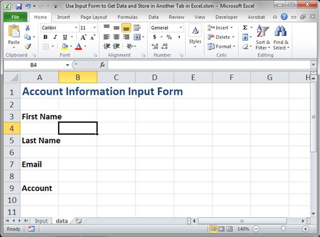
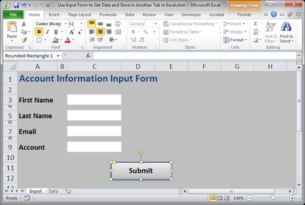
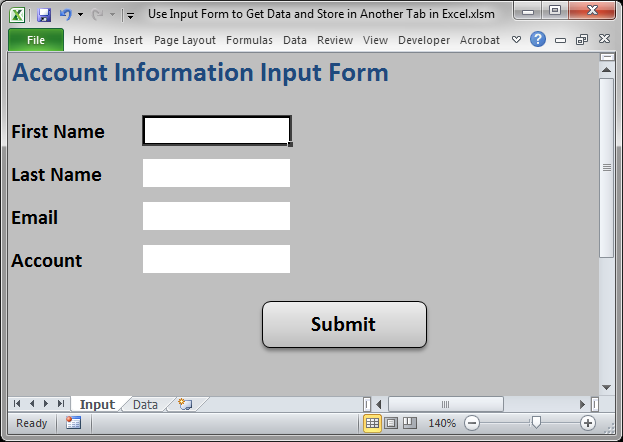
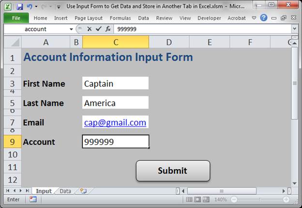
First, we create the form where the user will input the data. You can spend a lot of time or a little doing this but the most important thing is that it is easy for the user to understand what to do.
Here are some steps for a basic form that I like.
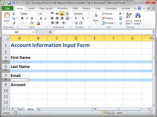
- Create a title and give it a title-like format:

- Skip a row and then input the form field’s titles. Skip a row between each form field. This allows you to control the spacing between the fields and that can make it easier to use.
Also apply some basic formatting to the title; I just make them bold. - Adjust the spacing between each field by selecting the empty row between them while holding the Ctrl button.
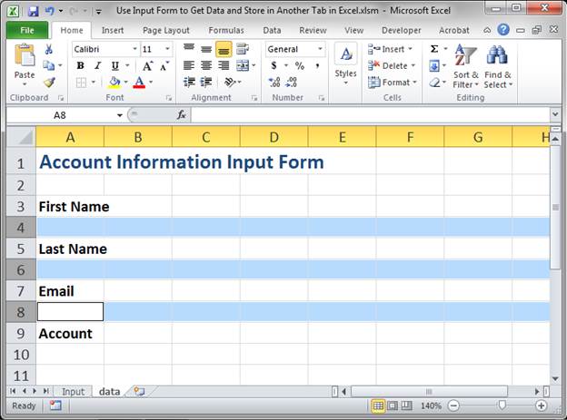
Then, change the height of one and all will change at the same time. - Make column A just big enough to show the titles for the form fields. Then make column B small; we will use this column as a separator between the form input field and title.
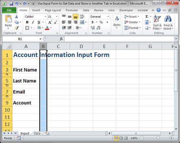
- Click the square in the upper left of the rows and columns or just hit Ctrl + A to select everything.
Click the paint bucket in the Font box on the Home tab and select a grayish color for the background.
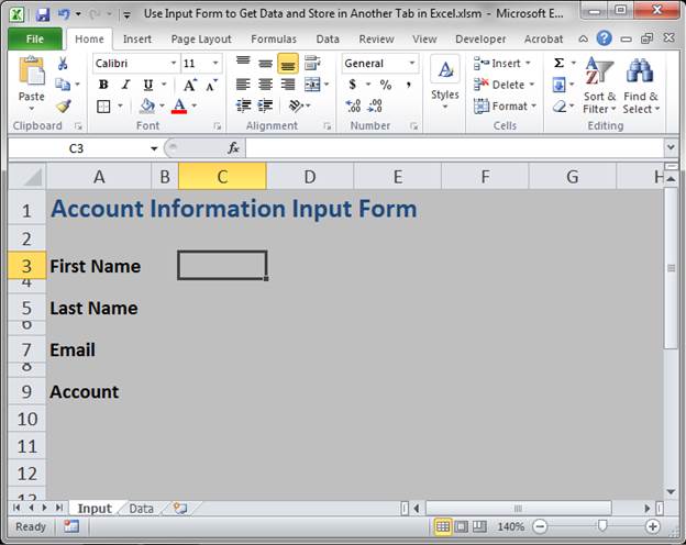
You will now have something like this: - Select the cells in column C that are in the same row as the form field titles and make their background white.
If you want, you can add a full border around each white cell; some people like that. - Time to add the button.
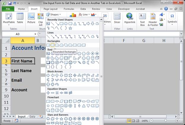
Go to the Insert tab and click Shapes and select a Rounded Rectangle from the list.
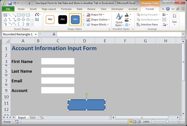
Then, left-click on the mouse, hold, and drag until you have the desired size for the button.
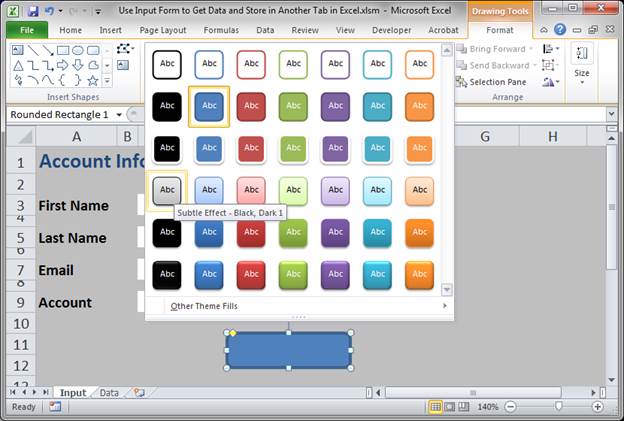
Make sure the button is selected and then go to the Format tab that will appear and click the bottom arrow in the Shape Styles section and select a pre-made one from there if you want.
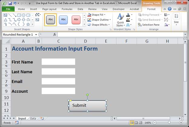
Click the button again and type some text.
Hit the Esc key when finished and then go to the Home tab and change the formatting of the text like you would regular text in a cell.
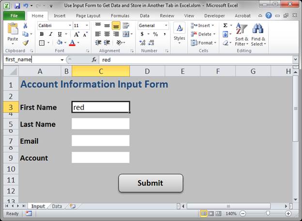
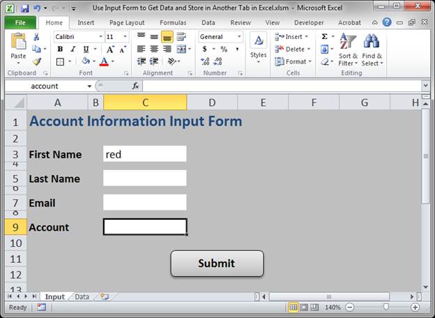
Now we have a pretty decent form. - Before we continue, I want to add a name to each input field. This will make creating the macro much easier.
Select the white input field for first name and then look to the white box just above where it says column A, that is the Name Box and that is where we will type a name for this field; I named mine first_name. Once you type the name, you must hit Enter. (hint: you can’t use spaces in the name)
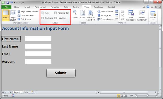
Repeat this for the other fields until each one has a unique name. - To finish the form’s appearance, go to the View tab and look in the Show section.
Uncheck Formula bar, Gridlines, and Headings. - Resize the window and hide the ribbon menu (you can use a macro to completely hide the ribbon menu if you want).
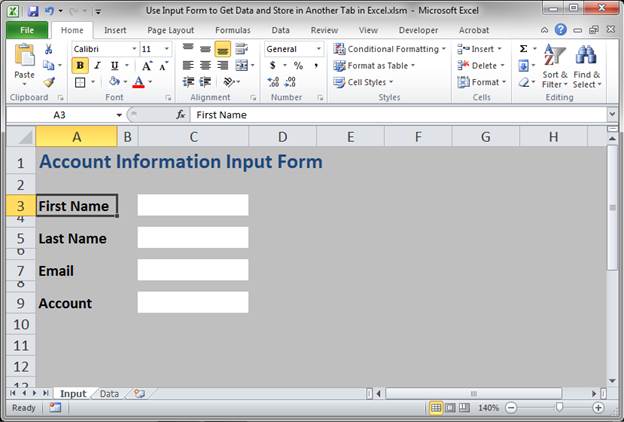
Now you’ve got a nice little form.
You can also lock the worksheet and leave only the 4 white input fields unlocked if you want to protect the form and you can use Data Validation to make sure the user inputs the correct type of data.
Create the Macro to Store the Data
Now that you have a form, let’s make that Submit button work.
Here, I will show you how to make a macro, but it will be easy to follow, I promise.
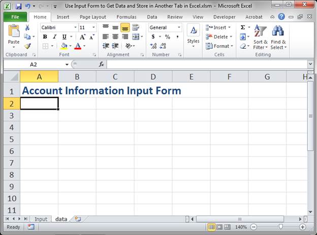
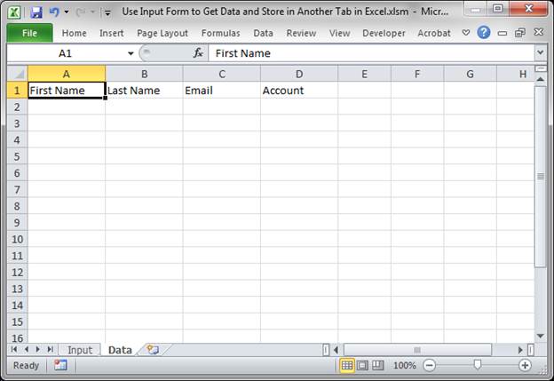
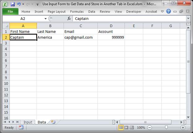
- Figure out where you will put the data. You can have it emailed somewhere, inserted into a real database, or simply stored on a separate worksheet. I’ll be covering the last option here, so the first step is to create the worksheet and make sure we know where the data will go.
I created a worksheet named Data and put a title for each column that will hold data.
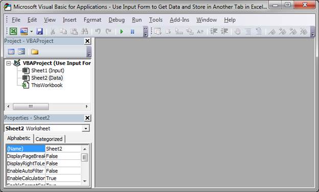
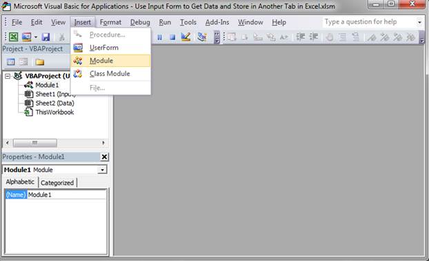
You also need to add a title row for your data in order for the macro I make here to work. - Time to create the macro. Hit Alt + F11 to go to the VBA window. It should look like this:
- Go to Insert > Module.
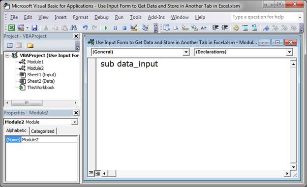
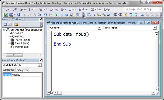
A blank window will open: - Type sub then a space and then the name you want to give the macro.
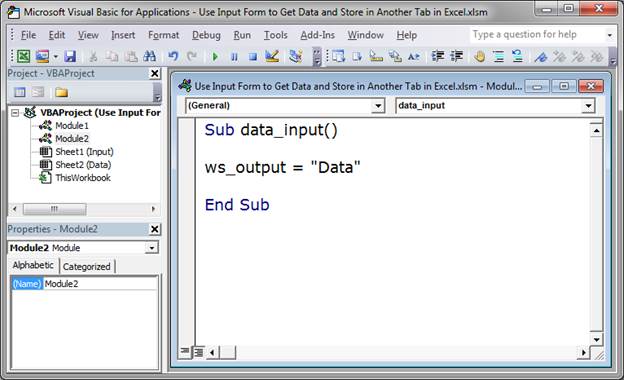
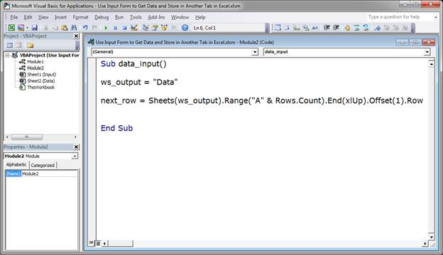
Hit Enter and it will automatically be formatted like this: - To start the macro, I store the name of the worksheet where the input will be stored, the Data worksheet. This is something that you don’t have to do but it will help a lot if you ever change the name of the worksheets.
The variable ws_output stores the text Data, which is just the name of the worksheet where the data will go.
(Since we gave a unique name to all of our input fields in Step 8 of the first section of this tutorial, we do not need to store the name of the data Input worksheet.) - Now, we need to find out what the next empty row on the data worksheet is so that we don’t overwrite anything.
This piece of code will find that row and store it into a variable named next_row:next_row = Sheets(ws_output).Range("A" & Rows.Count).End(xlUp).Offset(1).Row
This line of code can seem confusing but, to be honest, you don’t really need to know how it works except that ws_output needs to contain the name of the worksheet where you want to put the data and A is the column where you will put data that the user must always input; this column should not store optional data or you will end-up overwriting some data if the user chooses to leave that field blank.
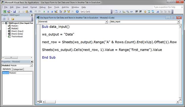
To learn more about this line of code, go to the tutorial here: find the next empty row in a worksheet - We now know where the data should go and where the next empty row is; next, we just need to take the data from the Input worksheet and put it into the Data worksheet.
Here is how it’s done with the First Name field.Sheets(ws_output).Cells(next_row, 1).Value = Range("first_name").Value
ws_output is the variable that stores the name of the Data worksheet.
Cells(next_row, 1) says where the data should go on the worksheet. next_row comes from the last step and says in which row the data will be placed. 1 is the column number where the data will go. The First Name value will go into column A and that is the first column, so a 1 goes there. For column B, we would use 2 instead of 1 and column C would be 3, etc.
Range(«first_name») is what selects the value from the first name cell on the Input worksheet. Since I named that cell first_name in step 8 of the first section of this tutorial, I do not have to reference the worksheet on which it is located; I can simply put the name of the cell inside Range() and it will get the correct value.
Value is in two places in this line of code and it is used to get the value of the first_name cell and to then put that value into the new cell on the Data worksheet.
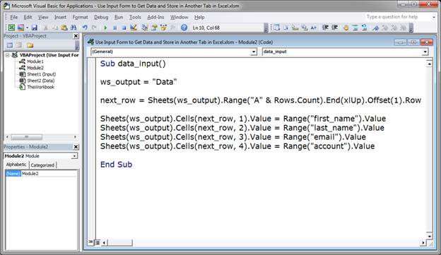
Here is the macro with the new line: - Repeat Step 7 for every piece of data that you want to store.
The three new lines here are:Sheets(ws_output).Cells(next_row, 2).Value = Range("last_name").Value Sheets(ws_output).Cells(next_row, 3).Value = Range("email").Value Sheets(ws_output).Cells(next_row, 4).Value = Range("account").Value
These lines will get the last name, email, and account values and put them onto the Data worksheet.
The only thing that is changed in each line is the column in which the data will be placed on the Data worksheet and the name of the cell from which we get the data.
To get the last name value from the Input worksheet, I put last_name in the range method: Range(«last_name»).
To put the last name value into the second column of the Data worksheet, I put a 2 into the cells method: Cells(next_row, 2).
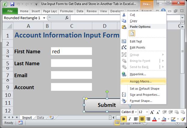
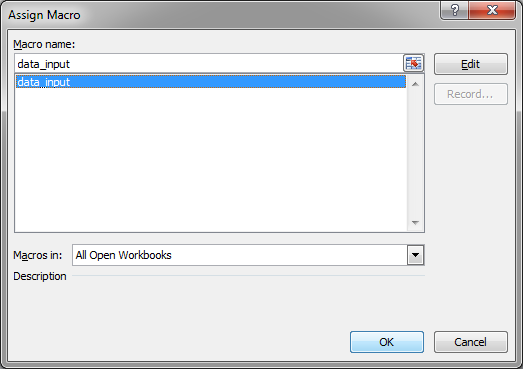
You can see that each line follows this pattern; the number of the column in the cells method is incremented by one, so each piece of data goes into the next column and the name of the cell in the range method is updated to get the desired piece of data. - Now, go back to Excel, Alt + F11, and attach the macro to the Submit button.
To do this, right-click the Submit button and click Assign Macro.
Select the macro from the list and click OK. - It’s time to test everything! Let’s input some data.
Click the Submit button, go to the Data tab, and you’ll see the data.
Whew, so that was a lot of steps, but you should now have a fully functioning Input form and data storage worksheet in Excel.
There are a number of other things you can add to the macro to make this a bit more user-friendly, such as clearing the form when a successful entry has been made, showing an output message that the data was stored, hiding and locking the Data worksheet so that a user can’t easily change it by hand, and more. But, what I have shown you here is the creation of the core functionality of the Input form and storage system. Get this working first and then proceed to add those other features. I will also cover many of those features in other tutorials.
Full Macro
If you just want the macro that I made for this tutorial, here it is:
Sub data_input()
ws_output = "Data"
next_row = Sheets(ws_output).Range("A" & Rows.Count).End(xlUp).Offset(1).Row
Sheets(ws_output).Cells(next_row, 1).Value = Range("first_name").Value
 Sheets(ws_output).Cells(next_row, 2).Value = Range("last_name").Value
 Sheets(ws_output).Cells(next_row, 3).Value = Range("email").Value
 Sheets(ws_output).Cells(next_row, 4).Value = Range("account").Value
End Sub
If you want a better understanding of this macro, read the section above called Create the Macro to Store the Data.
Notes
Not much to say about this one that I haven’t already said. I hope everything was clear and easy to understand but not too slow.
Make sure to download the workbook attached to this tutorial so you can get all of this in Excel (also, then you don’t have to start from scratch when building your own input form).
Similar Content on TeachExcel
Use a Form to Enter Data into a Table in Excel
Tutorial:
You can enter data into a table in Excel using a form; here I’ll show you how to do that….
Highlight, Sort, and Group the Top and Bottom Performers in a List in Excel
Tutorial:
How to highlight the rows of the top and bottom performers in a list of data.
This allows…
Get Data from Separate Workbooks in Excel
Tutorial: How to get data from separate workbooks in Excel. This tutorial includes an example using …
Formula to Get the Last Value from a List in Excel
Tutorial:
Formulas that you can use to get the value of the last non-empty cell in a range in Excel…
Loop through a Range of Cells in a UDF in Excel
Tutorial:
How to loop through a range of cells in a UDF, User Defined Function, in Excel. This is …
Excel Input Form with Macros and VBA
Tutorial:
Forms Course
How to make a data entry form in Excel using VBA and Macros — this allows yo…
Subscribe for Weekly Tutorials
BONUS: subscribe now to download our Top Tutorials Ebook!

Data Entry Forms is an extremely useful feature if inputting data is part of your daily work.
It can help you avoid the mistakes and make the data entry process faster. It also helps you focus on one record at a time!
It is a convenient and faster way to input records in Excel by displaying one row of information at a time without having to move from one column to another.
In this tutorial, we will show you How to Create Form in Excel for Data Entry.
Whenever I wanted to enter data in Excel, it would take me a very long time to input these records one by one, but I discovered a handy trick that can turn my Excel Table into a handy Excel Data Entry Form!

Say goodbye to inputting entering data into this Table row by row by row by row….
Below, we will cover the Top 11 Excel Data Entry Form Tips and Tricks that will be beneficial for you:
- #1 – Create Form in Excel
- #2 – Add to Quick Access Toolbar (QAT)
- #3 – Access the Form anytime
- #4 – Browse through Records
- #5 – Edit Existing Record
- #6 – Search Criteria
- #7 – Restore a Record
- #8 – Data Validation in Forms
- #9 – Delete a Record
- #10 – Close the Form
- #11 – Keyboard Shortcuts for Data Entry Forms
Make sure to download the Excel Workbook below and follow along:
DOWNLOAD EXCEL WORKBOOK
Want to know how to use the Data Entry Form?
*** Watch our video and step by step guide below with free downloadable Excel workbook to practice ***
Watch it on YouTube and give it a thumbs-up!
Watch it on YouTube and give it a thumbs-up!
Watch it on YouTube and give it a thumbs-up!
1. Create Form in Excel
I will show you how easy it is to Create Form in Excel for Data Entry with the following quick video below (scroll further down to see the step by step instructions after you watch this awesome video).
*** Watch our video below on How to Create Form in Excel in 5 minutes!***

DOWNLOAD OUR
FREE EXCEL GUIDES
In this tutorial, you have learned how to create form in Excel with minutes without using VBA!!
Follow the steps below:
STEP 1: Convert your Column names into a Table, go to Insert> Table
Make sure My table has headers is also checked.

STEP 2:Let us add the Form Creation functionality to understand how to make a fillable form in Excel.
Go to File > Options


STEP 3:Go to Customize Ribbon.
Select Commands Not in the Ribbon and Form. This is the functionality we need.
Click New Tab.

STEP 4:Under the New Tab, select New Group, and click Add.
This will add Forms to a New Tab in our Ribbon.

Notice that there is also a Rename button, you can use it to rename the New Tab and New Group into something more descriptive, like Form:

STEP 5:Select your Table, and on your new Form tab, select Form.

STEP 6: A new Form dialogue box will pop up!
Input your data into each section.
Click New to save it. Repeat this process for all the records you want to add.
Press Close to get out of this screen and see the data in your Excel Table.

You can now use this new form to continually input data into your Excel Table!

2. Add to Quick Access Toolbar (QAT)
Now that you have learned how to create form in Excel, lets put them on your QAT for easy access.
To add to the quick access toolbar, follow the steps below:
STEP 1: Click on the small arrow right next to QAT.

STEP 2: Click on More Commands from the dropdown list.

STEP 3: In the Excel Options dialog box, select All Commands from Choose commands from list.

STEP 4: Select Form from the list and then click on Add>>.

STEP 5: Form is now available in the Customize Quick Access Toolbar. Click OK.

Data Entry Form is now part of your Quick Access Toolbar.

3. Access the Form anytime
To access the Excel Data Entry Form, click on any cell in the table and click on the Form icon in Quick Access Toolbar.

If you try to access the form when you haven’t selected a cell within the data table, you will receive an error message like the one shown below:

4. Browse through Records
To navigate through the existing records, simply use the Find Previous and Find Next buttons available on the Data Entry Form.

You can also use the scroll bar to go through the records one after the other.

This will save time when you have a data with multiple columns and records.
5. Edit Existing Record
Use the Find Previous and Find Next buttons to search for the record to want to edit.
Once you find the desired record, simply make the necessary edit and hit Enter in Excel.

The data table will be updated with the changes made.

6. Search Criteria
Using Wildcards
If you wish to search all entries containing the word “east” in the Region Column, you can do that by using the wildcard asterisk (*).
STEP 1: In the Data Entry Form, click on the Criteria button

STEP 2: In the Region field, type *east (to search all-region containing the word east)

STEP 3: Click Find Next to find the entries containing the word east.

Excel Data Entry Form will find the three entries for you in this scenario!


Using greater or less than sign
If you want to search for persons having a salary greater than or equal to $75,000, you can do so by following the steps below:
STEP 1: In the Data Entry Form, click on the Criteria button
STEP 2: In the Salary field, type >=75000.

STEP 3: Click Find Next to find all entries with a salary greater than or equal to $75,000.


7. Restore a Record
Suppose you have accidentally deleted the first name of a record.

And you don’t remember what was written in that field! Don’t panic.
You can use the Restore button in the Excel Data Entry Form and retrieve the data lost accidentally.

The data will reappear in the respective field.

One thing you need to keep in mind is that the Restore button is only useful if you haven’t hit Enter.
The moment you press the Enter button, the Restore button will become inactive and you won’t be able to revert back to the original data.
8. Data Validation in Forms
Even though you cannot directly add any data validation to the form. Any restriction created on the data table will still be in effect in the Forms.
Let’s see how!
Say, you add a list rule to the Region Column using Data Validation.
STEP 1: Select the Region Column.

STEP 2: Go to Data Tab > Data Tools (Group) > Data Validation.

STEP 3: In the Data Validation dialog box, click on the Allow dropdown and select List.

STEP 4: In the Source field, type Northeast, Northwest, Southeast, Southwest, and click OK.

Data Validation has now been inserted in the Region Column where you are only allowed to enter values present in the list (Northeast, Northwest, Southeast, Southwest).
STEP 5: Click on the Forms icon in QAT.

STEP 6: Change the Region for Record 1 from Northeast to East and Click OK.

Once you click OK, you will see an error message as below:

9. Delete a Record

STEP 1: Use the Scroll Bar to navigate to find the entry you want to delete.
STEP 2: Simply, click on the Delete button.

STEP 3: A confirmation message will appear on your screen, Click OK.

The desired entry will be removed from the data table.

10. Close the Form
To close the dialog box for Data Forms, simply click on the Close button (X) on the top-right corner of the bix.

11. Keyboards Shortcuts for Data Entry Forms
You can use the following keyboard shortcuts to work faster when using Data Entry Forms:
- Press Tab to go to the next field in the Excel Forms.
- Press Enter to go to the next record in the Excel Forms.
- Hit the Esc button on your keyboard to close the Excel Form.
This completes our tutorial on the Top 11 things you should know if Data Entry is what you do in Excel. It will not only make the process faster but also a lot more easier and fun!
Few things to keep in mind when using the Excel Data Entry Form are:
- You can add a maximum of 32 fields per record.
- You cannot print a data form record.
- Before you hit Enter, you can restore any changes made to the data.
So, give it a try! I am sure you are gonna love it!!
You can know more about How to Create Form in Excel by going through this tutorial by Microsoft.
