Testing whether conditions are true or false and making logical comparisons between expressions are common to many tasks. You can use the AND, OR, NOT, and IF functions to create conditional formulas.
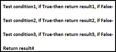
For example, the IF function uses the following arguments.

Formula that uses the IF function


For more information about how to create formulas, see Create or delete a formula.
What do you want to do?
-
Create a conditional formula that results in a logical value (TRUE or FALSE)
-
Create a conditional formula that results in another calculation or in values other than TRUE or FALSE
Create a conditional formula that results in a logical value (TRUE or FALSE)
To do this task, use the AND, OR, and NOT functions and operators as shown in the following example.
Example
The example may be easier to understand if you copy it to a blank worksheet.
How do I copy an example?
-
Select the example in this article.
Selecting an example from Help
-
Press CTRL+C.
-
In Excel, create a blank workbook or worksheet.
-
In the worksheet, select cell A1, and press CTRL+V.
Important: For the example to work properly, you must paste it into cell A1 of the worksheet.
-
To switch between viewing the results and viewing the formulas that return the results, press CTRL+` (grave accent), or on the Formulas tab, in the Formula Auditing group, click the Show Formulas button.
After you copy the example to a blank worksheet, you can adapt it to suit your needs.
|
For more information about how to use these functions, see AND function, OR function, and NOT function.
Top of Page
Create a conditional formula that results in another calculation or in values other than TRUE or FALSE
To do this task, use the IF, AND, and OR functions and operators as shown in the following example.
Example
The example may be easier to understand if you copy it to a blank worksheet.
How do I copy an example?
-
Select the example in this article.
Important: Do not select the row or column headers.
Selecting an example from Help
-
Press CTRL+C.
-
In Excel, create a blank workbook or worksheet.
-
In the worksheet, select cell A1, and press CTRL+V.
Important: For the example to work properly, you must paste it into cell A1 of the worksheet.
-
To switch between viewing the results and viewing the formulas that return the results, press CTRL+` (grave accent), or on the Formulas tab, in the Formula Auditing group, click the Show Formulas button.
After you copy the example to a blank worksheet, you can adapt it to suit your needs.
|
For more information about how to use these functions, see IF function, AND function, and OR function.
Top of Page
The logical IF statement in Excel is used for the recording of certain conditions. It compares the number and / or text, function, etc. of the formula when the values correspond to the set parameters, and then there is one record, when do not respond — another.
Logic functions — it is a very simple and effective tool that is often used in practice. Let us consider it in details by examples.
The syntax of the function «IF» with one condition
The operation syntax in Excel is the structure of the functions necessary for its operation data.
=IF(boolean;value_if_TRUE;value_if_FALSE)
Let us consider the function syntax:
- Boolean – what the operator checks (text or numeric data cell).
- Value_if_TRUE – what will appear in the cell when the text or numbers correspond to a predetermined condition (true).
- Value_if_FALSE – what appears in the box when the text or the number does not meet the predetermined condition (false).
Example:
Logical IF functions.
The operator checks the A1 cell and compares it to 20. This is a «Boolean». When the contents of the column is more than 20, there is a true legend «greater 20». In the other case it’s «less or equal 20».
Attention! The words in the formula need to be quoted. For Excel to understand that you want to display text values.
Here is one more example. To gain admission to the exam, a group of students must successfully pass a test. The results are listed in a table with columns: a list of students, a credit, an exam.
The statement IF should check not the digital data type but the text. Therefore, we prescribed in the formula В2= «done» We take the quotes for the program to recognize the text correctly.
The function IF in Excel with multiple conditions
Usually one condition for the logic function is not enough. If you need to consider several options for decision-making, spread operators’ IF into each other. Thus, we get several functions IF in Excel.
The syntax is as follows:
Here the operator checks the two parameters. If the first condition is true, the formula returns the first argument is the truth. False — the operator checks the second condition.
Examples of a few conditions of the function IF in Excel:
It’s a table for the analysis of the progress. The student received 5 points:
- А – excellent;
- В – above average or superior work;
- C – satisfactory;
- D – a passing grade;
- E – completely unsatisfactory.
IF statement checks two conditions: the equality of value in the cells.
In this example, we have added a third condition, which implies the presence of another report card and «twos». The principle of the operator is the same.
Enhanced functionality with the help of the operators «AND» and «OR»
When you need to check out a few of the true conditions you use the function И. The point is: IF A = 1 AND A = 2 THEN meaning в ELSE meaning с.
OR function checks the condition 1 or condition 2. As soon as at least one condition is true, the result is true. The point is: IF A = 1 OR A = 2 THEN value B ELSE value C.
Functions AND & OR can check up to 30 conditions.
An example of using the operator AND:
It’s the example of using the logical operator OR.
How to compare data in two tables
Users often need to compare the two spreadsheets in an Excel to match. Examples of the «life»: compare the prices of goods in different bringing, to compare balances (accounting reports) in a few months, the progress of pupils (students) of different classes, in different quarters, etc.
To compare the two tables in Excel, you can use the COUNTIFS statement. Consider the order of application functions.
For example, consider the two tables with the specifications of various food processors. We planned allocation of color differences. This problem in Excel solves the conditional formatting.
Baseline data (tables, which will work with):
Select the first table. Conditional Formatting — create a rule — use a formula to determine the formatted cells:

In the formula bar write: = COUNTIFS (comparable range; first cell of first table)=0. Comparing range is in the second table.
To drive the formula into the range, just select it first cell and the last. «= 0» means the search for the exact command (not approximate) values.
Choose the format and establish what changes in the cell formula in compliance. It’s better to do a color fill.
Select the second table. Conditional Formatting — create a rule — use the formula. Use the same operator (COUNTIFS). For the second table formula:
Download all examples in Excel
Now it is easy to compare the characteristics of the data in the table.
Conditional Statements in Excel VBA – If Else, Case, For, Do While, Do Until, Nested Ifs
Conditional Statements in Excel VBA are very useful in programming, this will give you to perform comparisons to decide or loop through certain number of iterations based on a criteria. In this tutorial we will learn the conditional statements with examples.

- In this tutorial:
- » IF Statement
- » If … Else Statement
- » If … ElseIf … Else Statement
- » If … ElseIf … ElseIf Statement
- » Nested If Statement
Conditional Statements in Excel VBA – Download: Example File
Download this example file, we will learn conditional statements with examples.
ANALYSISTABS Examples on Conditional Statements
IF Statement
If .. Then
Syntax:
If <Condition> Then <Statement>
It is a simple Condition to check an expression, if the condition is True it will execute the Statement.
Sub sb1_IFCondition()

     'Check if cell(C2)is greater than 6Lakhs
     If Range("C2") > 600000 Then Range("D2") = Range("C2") * 10 / 100

End Sub
(OR)
Sub sb1_IFCondition()

     'Check if cell(C2)is greater than 6Lakhs
     If Range("C2") > 600000 Then
         Range("D2") = Range("C2") * 10 / 100
     end if

End Sub
It will check if the range C2 value, if it is greater than 600000 it will execute the statement ‘Range(“D2”) = Range(“C2”) * 10 / 100’.
If … Else Statement
Syntax:
If <Condition> Then
   Statements1
Else
   Statements2
End if
It will check the Condition, if the condition is True it will execute the Statements1, if False execute the Statements2.
Example 1: Check whether the cell number is greater than six lakhs
Sub If_Else1()

If Range("B2") > 600000 Then
    Range("D2") = Range("C2") * 5 / 100
Else
    Range("D2") = Range("C2") * 10 / 100
End If

End Sub
Example 2: Check whether the number is even or odd
Sub If_Else2()

    'Variable declaration
    Dim Num As Integer

    'Accepting the number by the user
    Num = InputBox("Enter the Number:", "Number")

    If Num Mod 2 = 0 Then
        'Check whether the number is even
        MsgBox "Entered number is Even."
    Else
        'Check whether the number is odd
        MsgBox "Entered number is Odd."
    End If

End Sub
If … ElseIf … Else Statement
You can use If…ElseIf…Else to check more conditions:
If Condition1 Then
    Statements1
ElseIf Condition2 Then
    Statements2
Else
    StatementsN
End If
Example : Check whether the number entered by the user is positive, negative or equal to zero.
Sub If_ElseIf_Else()

    'Variable declaration
    Dim Num As Integer

    'Accepting the number by the user
    Num = InputBox("Enter the Number:", "Number")

    If Num < 0 Then
        'Check whether the number is less  than zero
        MsgBox "Number is negative."
    ElseIf Num = 0 Then
        'Check whether the number is equal to zero
        MsgBox "Number is zero."
    Else
        'Check whether the number is greater  than zero
        MsgBox "Number is positive."
    End If

End Sub
If … ElseIf … ElseIf Statement
You can use If…ElseIf…ElseIf to check more conditions:
If Condition1 Then
    Statements1
ElseIf Condition2 Then
    Statements2
ElseIf ConditionN Then
    StatementsN
End If
Example : Check whether the number entered by the user is positive, negative or equal to zero.
Sub If_ElseIf_ElseIf()

    'Variable declaration
    Dim Num As Integer

    'Accepting the number by the user
    Num = InputBox("Enter the Number:", "Number")

    If Num < 0 Then
        'Check whether the number is less  than zero
        MsgBox "Number is negative."
    ElseIf Num = 0 Then
        'Check whether the number is equal to zero
        MsgBox "Number is zero."
    ElseIf Num > 0 Then
        'Check whether the number is greater  than zero
        MsgBox "Number is positive."
    End If

End Sub
Nested If Statement
You can use If…ElseIf…ElseIf…ElseIf…Else to check more conditions:
If Condition1 Then
    Statements1
ElseIf Condition2 Then
    Statements2
ElseIf Condition3 Then
    Statements3

    ...........

ElseIf ConditionN Then
    StatementsN
End If
Example 1: Check if the month is fall under which quater using “Nested If” statement and “OR” Operator
Sub NestedIf_FindQuater()

    'Variable declaration
    Dim Mnt As String

    'Accepting the month by the user
    Mnt = InputBox("Enter the Month:", "Month")

    If Mnt = "January" Or Mnt = "February" Or Mnt = "March" Then
        'Check if the month is fall under first quater.
        MsgBox "First Quater."
    ElseIf Mnt = "April" Or Mnt = "May" Or Mnt = "June" Then
        'Check if the month is fall under second quater.
        MsgBox "Second Quater."
    ElseIf Mnt = "July" Or Mnt = "August" Or Mnt = "September" Then
        'Check if the month is fall under third quater.
        MsgBox "Third Quater."
    Else
        'Check if the month is fall under fourth quater.
        MsgBox "Fourth Quater."
    End If

End Sub
Example : Check Student Grade based on Marks using “Nested If” statement and “AND” operator
Sub NestedIf_StudentGrade()

    'Variable declaration
    Dim Mrks As String

    'Accepting the month by the user
    Mrks = InputBox("Enter the Marks:", "Marks")

    If Mrks <= 100 And Mrks >= 90 Then
        'Check if the Grade A++
        MsgBox "Grade : A++"
    ElseIf Mrks < 90 And Mrks >= 80 Then
        'Check if the Grade A+
        MsgBox "Grade : A+"
    ElseIf Mrks < 80 And Mrks >= 60 Then
        'Check if the Grade A
        MsgBox "Grade : A"
    ElseIf Mrks < 60 And Mrks >= 50 Then
        'Check if the Grade B
        MsgBox "Grade : B"
    ElseIf Mrks < 50 And Mrks >= 35 Then
        'Check if the Grade C
        MsgBox "Grade : C"
    Else
        'Check if the Grade has fail
        MsgBox "Grade : Fail"
    End If

End Sub
Select … Case
If you have a more number of conditions to check, the If condition will go through each one of them. The alternative of jumping to the statement that applies to the state of a condition is Select Case.
Syntax:
Select Case Expression
    Case Expression1
	Statement1
    Case Expression2
        Statement2
    Case ExpressionN
        StatementN
End Select
Following is the example on select case:
Sub sb3_SelectCaseCondition()
Select Case Range("B2")
    Case "D1"
    Range("D2") = Range("C2") * 10 / 100
    Case "D2"
    Range("D2") = Range("C2") * 20 / 100
    Case "D3", "D4"
    Range("D2") = Range("C2") * 15 / 100
    Case Else
    Range("D2") = Range("C2") * 5 / 100
End Select
End Sub
Loops
You can use loops to execute statements certain number of time or until it satisfies some condtion.
For Loop
For loop is useful to execute statements certain number of time.
Syntax:
For CounterVariable = Starting Number To Ending Number
  Statements
Next
The following example show you the message box 5 times with integers
Sub sbForLoop()
Dim iCntr  As Integer
For iCntr = 1 To 5
    msgbox iCntr
Next
End Sub
Following is another Example on For Loop:
Sub sb4_ForLoop()
Dim iCntr  As Integer
For iCntr = 2 To 16
    Cells(iCntr, 4) = Cells(iCntr, 3) * 10 / 100
Next
End Sub
You can use Step statement to stepping the counter.
Sub sbForLoop()
Dim iCntr  As Integer
For iCntr = 1 To 10 Step 2
    msgbox iCntr
Next
End Sub
By default the stepping counter is 1, the below two statements are same:
1. For iCntr = 1 To 10
2. For iCntr = 1 To 10 Step 1
For Each Item In the Loop
If you want to loop through a collection, you can use for each condition. The following example loop through the Sheets collection of the Workbook.
Sub sbForEachLoop()
Dim Sht As Worksheet
For Each Sht In ThisWorkbook.Sheets
    MsgBox Sht.Name
Next
End Sub
Do…While
Do loop is a technique used to repeat an action based on a criteria.
Syntax:
Do While Condition
  Statement(s)
Loop
It will execute the statements if the condition is true,The following is example on Dow While:
Sub sb5_DoWhileLoop()
Dim iCntr  As Integer
iCntr = 2
Do While Cells(iCntr, 3) <> ""
    Cells(iCntr, 4) = Cells(iCntr, 3) * 10 / 100
    iCntr = iCntr + 1
Loop
End Sub
Other flavors of the Do loop:
Do
    Statement(s)
Loop While Condition

'-------------------------------

Do
    Statements
Loop Until Condition

'-------------------------------

Do Until Condition
    Statement(s)
Loop
Exiting in between Loops and Procedure
You can Exit the For loop in between based on a condition using Exit For
In the following, it will exit the is for loop if the sheet name is equals to “Data”
Sub sbForEachLoop()
Dim Sht As Worksheet
For Each Sht In ThisWorkbook.Sheets
    MsgBox Sht.Name
    if Sht.Name="Data" then Exit For
Next
End Sub
You can Exit any Procedure using Exit Sub
In the following, it will exit the procedure if the sheet name is equals to “Data”
Sub sbForEachLoop()
Dim Sht As Worksheet
For Each Sht In ThisWorkbook.Sheets
    MsgBox Sht.Name
    if Sht.Name="Data" then Exit Sub
Next
End Sub
You can Exit Exiting a Do Loop using Exit Do
A Powerful & Multi-purpose Templates for project management. Now seamlessly manage your projects, tasks, meetings, presentations, teams, customers, stakeholders and time. This page describes all the amazing new features and options that come with our premium templates.
Save Up to 85% LIMITED TIME OFFER

All-in-One Pack
120+ Project Management Templates
Essential Pack
50+ Project Management Templates
Excel Pack
50+ Excel PM Templates
PowerPoint Pack
50+ Excel PM Templates
MS Word Pack
25+ Word PM Templates
Ultimate Project Management Template
Ultimate Resource Management Template
Project Portfolio Management Templates
Related Posts
-
- Conditional Statements in Excel VBA – Download: Example File
- You can use Step statement to stepping the counter.
- You can Exit the For loop in between based on a condition using Exit For
- You can Exit any Procedure using Exit Sub
- You can Exit Exiting a Do Loop using Exit Do
- Conditional Statements in Excel VBA – Download: Example File
VBA Reference
Effortlessly
Manage Your Projects
120+ Project Management Templates
Seamlessly manage your projects with our powerful & multi-purpose templates for project management.
120+ PM Templates Includes:
6 Comments
-
I read a lot of interesting articles here. Probably you
spend a lot of time writing, i know how to save you a lot of time, there is an online tool
that creates high quality, SEO friendly articles in minutes, just search
in google – laranitas free content source -
Daniel Hill
May 6, 2015 at 2:36 AM — ReplyCan you tell me why this code doesn’t work? I can’t get a For … Next or other versions to work either. For this code I get the following error message “Code execution has been interrupted”. Debug shows the problem is on the iCtr = iCtr + 1 line. Value in Cell(102,4) is dependent on value in cell (102,7).
iCtr = 1
Do Until Cells(102, 4) < 100
Cells(102, 7) = iCtr
iCtr = iCtr + 1
Loop -
Daniel Hill
May 6, 2015 at 2:45 AM — Reply -
Abhishek
June 28, 2015 at 5:07 PM — ReplyPlease add some examples of do until loop..
-
krishna singh
July 26, 2015 at 9:06 PM — ReplyHi Sir,
I am Trying to create a VBA for the Bank reconciliation Statement though some what i have succeed by viewing your clips but stuck in one problem
if suppose there are 2 sheets such as sheet 1 and sheet 2 . if chq and amount matched so how would we give the sr no in the both sheet which should be same and for the next match it should give other noRegards
Krishna -
Ruchi Sharma
January 12, 2018 at 4:47 PM — ReplyHi,
could you please help me out with the VBA code for a data which is in column A with numbers that starts from 1,2,3,4…
how can using VBA i can get numbers that starts from 1 and 2 stated as ‘balance sheet’ in column Bso in short i want data in column B from A basis some condition and that condition is that number in column A should starts from 1 and 2 only.
Please help!
Effectively Manage Your
Projects and Resources
ANALYSISTABS.COM provides free and premium project management tools, templates and dashboards for effectively managing the projects and analyzing the data.
We’re a crew of professionals expertise in Excel VBA, Business Analysis, Project Management. We’re Sharing our map to Project success with innovative tools, templates, tutorials and tips.
Project Management
Excel VBA
Download Free Excel 2007, 2010, 2013 Add-in for Creating Innovative Dashboards, Tools for Data Mining, Analysis, Visualization. Learn VBA for MS Excel, Word, PowerPoint, Access, Outlook to develop applications for retail, insurance, banking, finance, telecom, healthcare domains.
Page load link
Go to Top
Multiple IF Conditions in Excel
The multiple IF conditions in Excel are IF statements contained within another IF statement. They are used to test multiple conditions simultaneously and return distinct values. The additional IF statements can be included in the “value if true” and “value if false” arguments of a standard IF formula.
For example, suppose we have a dataset of students’ scores from B1:B12. We need to grade the students according to their scores. Then, using the IF condition, we can manage the multiple conditions. In this example, we can insert the nested IF formula in cell D1 to assign a grade to a score. We can grade total score as “A,” “B,” “C,” “D,” and “F.” A score would be “F” if it is greater than or equal to 30, “D” if it is greater than 60, and “C” if it is greater than or equal to 70, and “A,” “B” if the score is less than 95. We can insert the formula in D1 with 5 separate IF functions:
=IF(B1>30,”F”,IF(B1>60,”D”,IF(B1>70,”C”,IF(C5>80,”B”,”A”))))
Table of contents
- Multiple IF Condition in Excel
- Explanation
- Examples
- Example #1
- Example #2
- Example #3
- Example #4
- Things to Remember
- Recommended Articles
Explanation
The IF formula is used when we wish to test a condition and return one value if the condition is met and another value if it is not met.
Each subsequent IF formula is incorporated into the “value_if_false” argument of the previous IF. So, the nested IF excelIn Excel, nested if function means using another logical or conditional function with the if function to test multiple conditions. For example, if there are two conditions to be tested, we can use the logical functions AND or OR depending on the situation, or we can use the other conditional functions to test even more ifs inside a single if.read more formula works as follows:
Syntax
IF (condition1, result1, IF (condition2, result2, IF (condition3, result3,………..)))
Examples
You can download this Multiple Ifs Excel Template here – Multiple Ifs Excel Template
Example #1
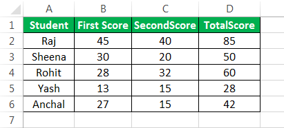
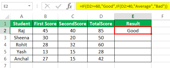
Suppose we wish to find how a student scores in an exam. There are two exam scores of a student, and we define the total score (sum of the two scores) as “Good,” “Average,” and “Bad.” A score would be “Good” if it is greater than or equal to 60, ‘Average’ if it is between 40 and 60, and ‘Bad’ if it is less than or equal to 40.
Let us say the first score is stored in column B, the second in column C.
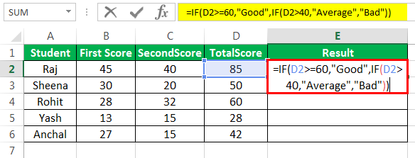
The following formula tells Excel to return “Good,” “Average,” or “Bad”:
=IF(D2>=60,”Good”,IF(D2>40,”Average”,”Bad”))
This formula returns the result as given below:
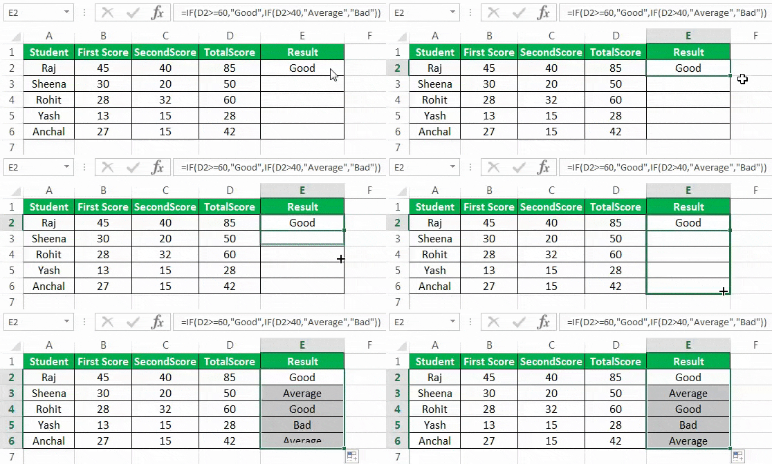
Drag the formula to get results for the rest of the cells.
We can see that one multiple IF function is sufficient in this case as we need to get only 3 results.
We can see that one multiple IF function is sufficient in this case as we need to get only 3 results.
Example #2
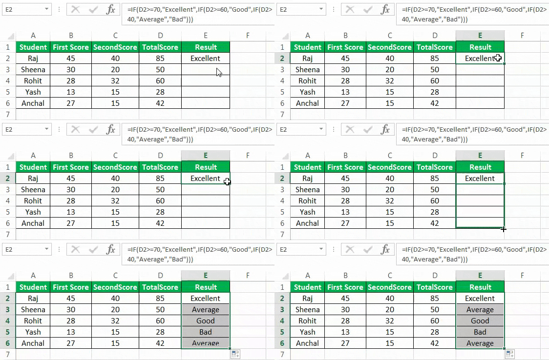
We want to test one more condition in the above examples: the total score of 70 and above is categorized as “Excellent.”
=IF(D2>=70,”Excellent”,IF(D2>=60,”Good”,IF(D2>40,”Average”,”Bad”)))
This formula returns the result as given below:
Excellent: >=70
Good: Between 60 & 69
Average: Between 41 & 59
Bad: <=40
Drag the formula to get results for the rest of the cells.
We can add several “IF” conditions if required similarly.
Example #3
Suppose we wish to test a few sets of different conditions. In that case, those conditions can be expressed using logical OR and AND, nesting the functions inside IF statements and then nesting the IF statements into each other.
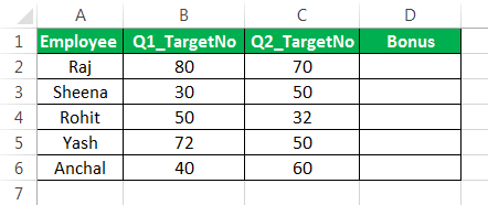
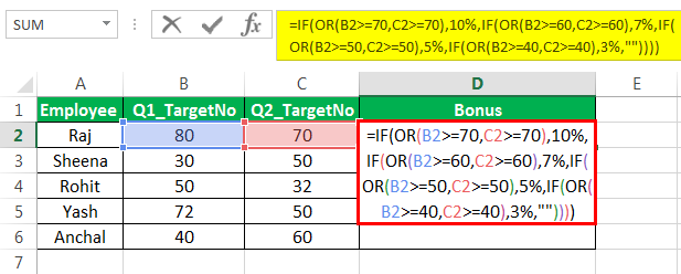
For instance, if we have two columns containing the number of targets made by an employee in 2 quarters: Q1 and Q2. Then, we wish to calculate the performance bonus of the employee based on a higher target number.
We can make a formula with the logic:
- If either Q1 or Q2 targets are greater than 70, then the employee gets a 10% bonus,
- If either of them is greater than 60, then the employee receives a 7% bonus,
- If either of them is greater than 50, then the employee gets a 5% bonus,
- If either is greater than 40, then the employee receives a 3% bonus. Else, no bonus.
So, we first write a few OR statements like (B2>=70,C2>=70), and then nest them into logical tests of IF functions as follows:
=IF(OR(B2>=70,C2>=70),10%,IF(OR(B2>=60,C2>=60),7%, IF(OR(B2>=50,C2>=50),5%, IF(OR(B2>=40,C2>=40),3%,””))))
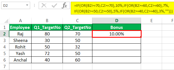
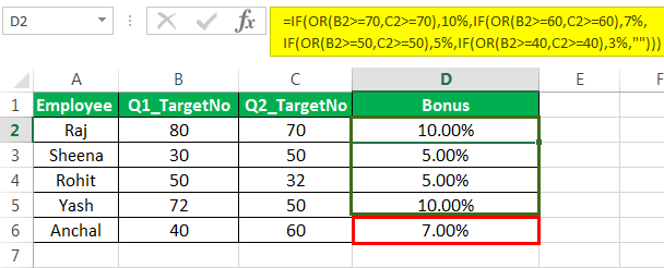
This formula returns the result as given below:
Next, drag the formula to get the results of the rest of the cells.
Example #4
Now, let us say we want to test one more condition in the above example:
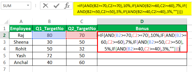
- If both Q1 and Q2 targets are greater than 70, then the employee gets a 10% bonus
- if both of them are greater than 60, then the employee receives a 7% bonus
- if both of them are greater than 50, then the employee gets a 5% bonus
- if both of them are greater than 40, then the employee receives a 3% bonus
- Else, no bonus.
So, we first write a few AND statements like (B2>=70,C2>=70), and then nest them: tests of IF functions as follows:
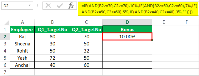
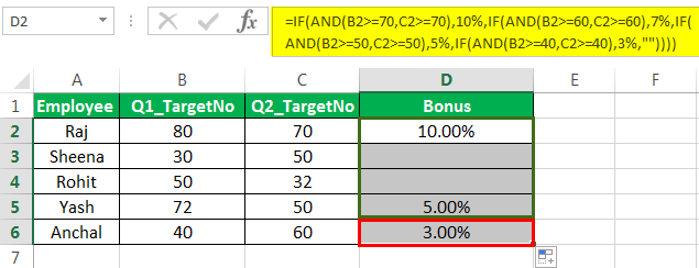
=IF(AND(B2>=70,C2>=70),10%,IF(AND(B2>=60,C2>=60),7%, IF(AND(B2>=50,C2>=50),5%, IF(AND(B2>=40,C2>=40),3%,””))))
This formula returns the result as given below:
Next, drag the formula to get results for the rest of the cells.
Things to Remember
- The multiple IF function evaluates the logical tests in the order they appear in a formula. So, for example, as soon as one condition evaluates to be “True,” the following conditions are not tested.
- For instance, if we consider the second example discussed above, the multiple IF condition in Excel evaluates the first logical test (D2>=70) and returns “Excellent” because the condition is “True” in the below formula:
=IF(D2>=70,”Excellent”,IF(D2>=60,,”Good”,IF(D2>40,”Average”,”Bad”))
Now, if we reverse the order of IF functions in Excel as follows:
=IF(D2>40,”Average”,IF(D2>=60,,”Good”,IF(D2>=70,”Excellent”,”Bad”))
In this case, the formula tests the first condition. Since 85 is greater than or equal to 70, a result of this condition is also “True,” so the formula would return “Average” instead of “Excellent” without testing the following conditions.
Correct Order
Incorrect Order
Note: Changing the order of the IF function in Excel would change the result.
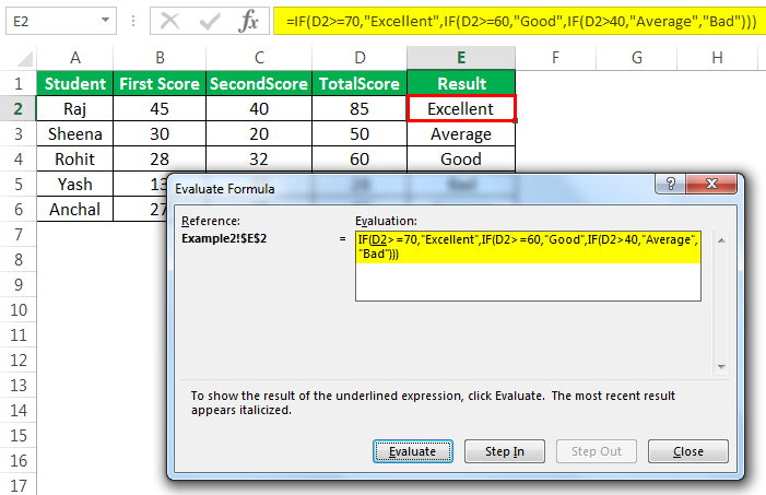
- Evaluate the formula logic– To see the step-by-step evaluation of multiple IF conditions, we can use the ‘Evaluate Formula’ feature in excel on the “Formula” tab in the “Formula Auditing” group. Clicking the “Evaluate” button will show all the steps in the evaluation process.
- For instance, in the second example, the evaluation of the first logical testA logical test in Excel results in an analytical output, either true or false. The equals to operator, “=,” is the most commonly used logical test.read more of multiple IF formulas will go as D2>=70; 85>=70; True; Excellent.
- Balancing the parentheses: If the parentheses do not match in terms of number and order, then the multiple IF formula would not work.
- If we have more than one set of parentheses, the parentheses pairs are shaded in different colors so that the opening parentheses match the closing ones.
- Also, on closing the parenthesis, the matching pair is highlighted.
- Numbers and Text should be treated differently: The text should always be enclosed in double quotes in the multiple IF formula.
- Multiple IF’s can often become troublesome: Managing many true and false conditions and closing brackets in one statement becomes difficult. Therefore, it is always good to use other tools like IF function or VLOOKUP in case Multiple IF’sSometimes while working with data, when we match the data to the reference Vlookup, it finds the first value and does not look for the next value. However, for a second result, to use Vlookup with multiple criteria, we need to use other functions with it.read more are difficult to maintain in Excel.
Recommended Articles
This article is a guide to Multiple IF Conditions in Excel. We discuss using multiple IF conditions, practical examples, and a downloadable Excel template. You may also learn more about Excel from the following articles: –
- IF OR in VBAIF OR is not a single statement; it is a pair of logical functions used together in VBA when we have more than one criteria to check, and when we use the if statement, we receive the true result if either of the criteria is met.read more
- COUNTIF in ExcelThe COUNTIF function in Excel counts the number of cells within a range based on pre-defined criteria. It is used to count cells that include dates, numbers, or text. For example, COUNTIF(A1:A10,”Trump”) will count the number of cells within the range A1:A10 that contain the text “Trump”
read more - IFERROR Excel Function – ExamplesThe IFERROR function in Excel checks a formula (or a cell) for errors and returns a specified value in place of the error.read more
- SUMIF Excel FunctionThe SUMIF Excel function calculates the sum of a range of cells based on given criteria. The criteria can include dates, numbers, and text. For example, the formula “=SUMIF(B1:B5, “<=12”)” adds the values in the cell range B1:B5, which are less than or equal to 12.
read more
The IF function is one of the most commonly used in Excel. The function can test a single condition as well as perform multiple complex logic tests. We can thus control the execution of Excel tasks using the IF function.
This is important since it enables us to perform actions depending on whether they meet certain conditions defined by the IF formula. We can also add data to cells using the function if other cells meet any of the conditions defined in the IF formula.
To add multiple conditions to an IF formula, we simply add nested IF functions.
In this article, you will learn the basics of the IF function and how to come up with an array of IF formulas. You will also learn the nested IF’s function.
Let’s get started!
1. Basic IF formula that tests a single condition
A single IF statement tests whether a condition is met and returns a value if TRUE and another value if FALSE.
IF (logical test, ‘value_if_true’, ‘value_if_false’)
In the example below, let us test whether the price is less than or equal to 2000. If the condition is true return cheap, otherwise return expensive!
Go to Cell C2 and type ‘=IF(B2<=2000,»CHEAP», «EXPENSIVE»)’
The if formula above records or posts the String Good whenever the single condition B2<=2000.
2. IF formula with multiple conditions (Nested IF Functions.
If you have complex data or want to perform powerful data analysis, you might need to test multiple conditions at a time. You might need to perform a logical test across multiple conditions.
In such cases, you have to use an IF statement with multiple conditions/ranges in a single formula. These multiple IF conditions are normally called nested IF Functions. The function is used if want more than 3 different results.
The general syntax for IF function with multiple conditions is
=IF (condition one is true, do something, IF (condition two is true, do something, IF (conditions three is true, do something, else do something)))
Commas are used to separate conditions and IF functions in the IF formula. The «)» is used to close all IFs at the End of the formula while the » (» opens all IF functions. The number of «(» should be equal to that of «)».
In our above example, we can include multiple conditions in the IF formula as follows
=IF(B2<=2000,»CHEAP»,IF(B2<=6000,»AFFORDABLE»,IF(B2<=10000,»EXPENSIVE»,»LUXURIOUS»)))
Press Enter to get the results and use the AutoFill feature to copy the formula to the rest of the cells.
3. IF formula with logical test
You can use an IF statement with AND and OR conditions to perform a logical test. IF your formula has AND function, the logical test returns TRUE if all the conditions are met; otherwise, it will return FALSE. While the OR Function returns TRUE if any of the conditions is met; otherwise it returns FALSE.
3.1 IF with AND Function
In the example below, a student is deemed to pass the exam if he/she has a score of 42 in Maths and 50 in English.
With this information, we can write the condition as follows;
AND (C14>=42, D14>=50)
To know whether the student passed or failed the exam. You can use the IF statement.
= IF(AND (C14>=42, D14>=50),”PASS”,”FAIL”)
Press enter and use the AutoFill feature to copy the formula to the rest of the cells.
3.2 IF with OR Function
The IF with OR Function works the same way as the AND function we have seen above. The only difference is that, if one of the conditions is TRUE then the result will be TRUE.
Follow the above process to apply the OR Function.
In cell E14, type = IF(OR (C14>=42, D14>=50),”PASS”,”FAIL”)
Press enter to get the results.
3. IF with ISNUMBER and ISTEXT Functions
You can use ISNUMBER and ISTEXT formula to find whether the cells have text value, number, or blank.
=IF(ISTEXT(A1), «Text», IF(ISNUMBER(A1), «Number», IF(ISBLANK(A1), «Blank», «»)))
You can only apply AND & OR functions at a time if your task requires you to evaluate several sets of conditions. For example, if you are checking exam results using these criteria:
Condition 1: exam1>50 and exam2>50
Condition 2: exam1>40 and exam2>60
In this case, the exam is deemed passed if either of the conditions is passed.
Although the formula may seem tricky, you only need to express each condition as an AND statement and nest them in the OR function. That is because meeting all the conditions is not necessary, but either statement will serve the purpose. Therefore, the general formula will be:
OR(AND(B2>50, C2>50), AND(B2>40, C2>60)
You can now use the OR function to test the logic of IF and supply the desired value_if_true and value_if_false values. In the end, the final IF formula with multiple AND & OR statements will turn into:
=IF(OR(AND(B2>50, C2>50), AND(B2>40, C2>60), «Pass», «Fail»)
5. Using the Array Formula
An Array formula can also help to get an Excel IF to test multiple conditions. For example, to evaluate the AND logical condition, you can use the asterisk:
IF(condition1) * (condition2) * …, value_if_true, value_if_false)
While to test conditions using OR logic, you will apply the plus sign:
IF(condition1) + (condition2) + …, value_if_true, value_if_false)
Finally, you can complete the Array formula by pressing Ctrl + Shift + Enter buttons together. The trick can also work as a regular formula in Excel 365 and Excel 2021 since it supports dynamic arrays.
Example: We can get “Pass” if cells B2 and C2 are greater than 50 by applying the formulas;
=IF((B2>50) * (C2>50), «Pass», «Fail») for AND logic
…, and
=IF((B2>50) + (C2>50), «Pass», «Fail») for OR logic.
6. IF With Other Excel Functions
Other Excel functions that can give the IF formula for multiple conditions include
6.1 IF#N/A Error in VLOOKUP Function
The VLOOKUP or any other lookup function returns a N/A error if it cannot find something. Therefore, you can return zero, blank, or text if #N/A to make your table neat. Here, you will need the following generic formula:
IF(ISNA(VLOOKUP(…)), value_if_na, VLOOKUP(…))
Example 1. If the lookup value in a cell (E1) is not found, the formula returns 0 as shown below;
=IF(ISNA(VLOOKUP(E1, A2:B10, 2,FALSE )), 0, VLOOKUP(E1, A2:B10, 2, FALSE))
Example 2: If the lookup value is not found, the formula returns blank as shown below;
=IF(ISNA(VLOOKUP(E1, A2:B10, 2,FALSE )), «», VLOOKUP(E1, A2:B10, 2, FALSE))
Example 3: If the lookup value is not available, the formula returns a specific text as shown below;
=IF(ISNA(VLOOKUP(E1, A2:B10, 2,FALSE )), «Not found», VLOOKUP(E1, A2:B10, 2, FALSE))
6.2 IF With SUM, AVERAGE, MIN, and MAX Functions
Excel has the SUMIF and SUMIFS functions that you can use, to sum up values in cells using certain criteria. You can use the SUM function to test the IF logic of your business. For instance, you can apply this formula to determine the text labels based on the sum of cells B2 and C2 values;
=IF(SUM(B2:C2)>130, «Good», IF(SUM(B2:C2)>110, «Satisfactory», «Poor»))
From the formula, the return text label is “Good” if the sum of the two cells is greater than 130. If the sum is greater than 110, the return text is “Satisfactory”, while if the sum is 110 or below, the return text is “Poor”.
You can still embed the AVERAGE function similarly to test the IF logic and return a different text label based on the average score of the two cells. In this case, the generic formula will be;
=IF(AVERAGE(B2:C2)>65, «Good», IF(AVERAGE(B2:C2)>55, «Satisfactory», «Poor»))
If the sum of cells B2 and C2 is indicated in cell D2, you can use the MAX and MIN functions to identify the highest and lowest values through the formulas;
=IF(D2=MAX($D$2: $D$10), «Best result», «»)
=IF(D2=MAX($D$2: $D$10), «Best result», «»)
Lastly, you can nest the two functions into one another to have both text labels in one column to get the formula;
=IF(D2=MAX($D$2:$D$10), «Best result», IF(D2=MIN($D$2:$D$10), «Worst result», «»))
6.3 IF with CONCATENATE Function
You can also use the CONCATENATE and IF functions to output the result of IF and some text into one cell. Here, you can use the formula;
=CONCATENATE(«You performed «, IF(B1>100,»fantastic!», IF(B1>50, «well», «poor»)))
From the formula, the student will get a «fantastic» result if the score in cell B1 is greater than 100. On the other hand, the result will be «well» if the score in cell B1 is greater than 50.
6.4 IF with ISERROR and ISNA Functions
These functions can only work in modern Excel versions where they trap and replace errors with another predefined value. For instance, the IFERROR function works in Excel 2007 and later, while the IFNA function works in Excel 2013 and later. When using earlier Excel versions, you will need the combinations of IF ISERROR and IF ISNA. So, what is the difference between these applications?
The answer is simple: IFERROR and ISERROR functions can handle all the possible errors resulting from Excel calculations, including VALUE, N/A, NAME, REF, NUM, DIV/0, and NULL errors. Contrary, IFNA, and ISNA handle only N/A errors.
Example: If you want to replace the #DIV/0 (divide by zero error) with a predefined text or value, you can use the formula;
=IF(ISERROR(A2/B2), «N/A», A2/B2), where;
A2 represents the value in cell A2
B2 represents the value in cell B2.
A2/B2 represents the results attained after dividing A2 by B2.
If the value in cell B2 is 0, the formula will return a N/A text.
I hope you found this tutorial useful.

