
Excel for Microsoft 365 Excel 2021 Excel 2019 Excel 2016 Excel 2013 Excel 2010 Excel 2007 More…Less
You can make the data on your worksheets more visible by changing the font color of cells or a range of cells, formatting the color of worksheet tabs, or changing the color of formulas.
For information on changing the background color of cells, or applying patterns or fill colors, see Add or change the background color of cells.
Change the text color for a cell or range of cells
-
Select the cell or range of cells that has the data you want to format. You can also select just a portion of the text within a cell.
-
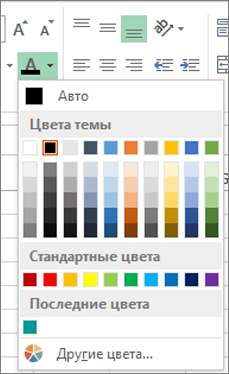
On the Home tab, choose the arrow next to Font Color
 .
. -
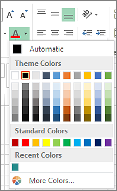
Under Theme Colors or Standard Colors, choose a color.
Tip: To apply the most recently selected text color, on the Home tab, choose Font Color.
Apply a custom color
If you want a specific font color, here’s how you can blend your custom color:
-
Click Home > Font Color arrow
> More Colors. -
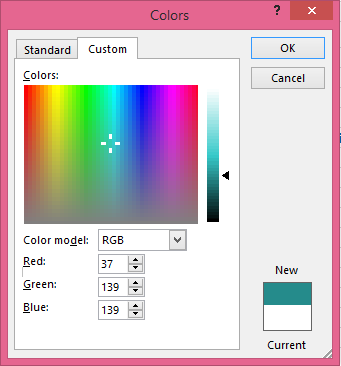
On the Custom tab, in the Colors box, select the color you want.
If you know the color numbers of a specific color, pick RGB (Red, Green, Blue) or HSL (Hue, Sat, Lum) in the Color model box, and then enter the numbers to match the exact color shade you want.
Tip: To quickly copy a font color you used to other cells, select a cell with that font color, and double-click Format Painter  . Then click the cells you want to format. When you’re done, click Format Painter again to turn it off.
Format the color of a worksheet tab
-
Right-click the worksheet tab whose color you want to change.
-
Choose Tab Color, and then select the color you want.
The color of the tab changes, but not the color of the font. When you choose a dark tab color, the font switches to white, and when you choose a light color for the tab, the font switches to black.
Need more help?
Want more options?
Explore subscription benefits, browse training courses, learn how to secure your device, and more.
Communities help you ask and answer questions, give feedback, and hear from experts with rich knowledge.
Изменение цвета текста (шрифта) в ячейке рабочего листа Excel с помощью кода VBA. Свойства ячейки (диапазона) .Font.Color, .Font.ColorIndex и .Font.TintAndShade.
Использование цветовой палитры для присвоения цвета тексту в ячейке листа Excel аналогично присвоению цвета фону ячейки, только свойство диапазона .Interior меняем на свойство .Font.
Цвет текста и предопределенные константы
Цвет шрифту в ячейке можно присвоить с помощью предопределенных констант:
|
Range(«A1:C3»).Font.Color = vbGreen Range(Cells(4, 1), Cells(6, 3)).Font.Color = vbBlue Cells(7, 1).Font.Color = vbRed |
Напомню, что вместо индексов строк и столбцов можно использовать переменные. Список предопределенных констант смотрите здесь.
Цвет шрифта и модель RGB
Для изменения цвета текста в ячейке можно использовать цветовую модель RGB:
|
Range(«A1»).Font.Color = RGB(200, 150, 250) Cells(2, 1).Font.Color = RGB(200, 150, 100) |
Аргументы функции RGB могут принимать значения от 0 до 255. Если все аргументы равны 0, цвет — черный, если все аргументы равны 255, цвет — белый. Функция RGB преобразует числовые значения основных цветов (красного, зеленого и синего) в индекс основной палитры.
Список стандартных цветов с RGB-кодами смотрите в статье: HTML. Коды и названия цветов.
Свойство .Font.ColorIndex
Свойство .Font.ColorIndex может принимать значения от 1 до 56. Это стандартная ограниченная палитра, которая существовала до Excel 2007 и используется до сих пор. Посмотрите примеры:
|
Range(«A1:D6»).Font.ColorIndex = 5 Cells(1, 6).Font.ColorIndex = 12 |
Таблица соответствия значений ограниченной палитры цвету:

Стандартная палитра Excel из 56 цветов
Подробнее о стандартной палитре Excel смотрите в статье: Стандартная палитра из 56 цветов.
Свойство .Font.ThemeColor
Свойство .Font.ThemeColor может принимать числовые или текстовые значения констант из коллекции MsoThemeColorIndex:
|
Range(«A1»).Font.ThemeColor = msoThemeColorHyperlink Cells(2, 1).Font.ThemeColor = msoThemeColorAccent4 |
Основная палитра
Основная палитра, начиная c Excel 2007, состоит из 16777216 цветов. Свойство .Font.Color может принимать значения от 0 до 16777215, причем 0 соответствует черному цвету, а 16777215 — белому.
|
Cells(1, 1).Font.Color = 0 Cells(2, 1).Font.Color = 6777215 Cells(3, 1).Font.Color = 4569325 |
Отрицательные значения свойства .Font.Color
При записи в Excel макрорекордером макроса с присвоением шрифту цвета используются отрицательные значения свойства .Font.Color, которые могут быть в пределах от -16777215 до -1. Отрицательные значения соответствуют по цвету положительному значению, равному сумме наибольшего индекса основной палитры и данного отрицательного значения. Например, отрицательное значение -8257985 соответствует положительному значению 8519230, являющегося результатом выражения 16777215 + (-8257985). Цвета текста двух ячеек из следующего кода будут одинаковы:
|
Cells(1, 1).Font.Color = —8257985 Cells(2, 1).Font.Color = 8519230 |
Свойство .Font.TintAndShade
Еще при записи макроса с присвоением шрифту цвета макрорекордером добавляется свойство .Font.TintAndShade, которое осветляет или затемняет цвет и принимает следующие значения:
- -1 — затемненный;
- 0 — нейтральный;
- 1 — осветленный.
При тестировании этого свойства в Excel 2016, сравнивая затемненные и осветленные цвета, разницы не заметил. Сравните сами:
|
Sub Test() With Range(Cells(1, 1), Cells(3, 1)) .Value = «Сравниваем оттенки» .Font.Color = 37985 End With Cells(1, 1).Font.TintAndShade = —1 Cells(2, 1).Font.TintAndShade = 0 Cells(3, 1).Font.TintAndShade = 1 End Sub |
В первые три ячейки первого столбца записывается одинаковый текст для удобства сравнения оттенков.
Разноцветный текст в ячейке
Отдельным частям текста в ячейке можно присвоить разные цвета. Для этого используется свойство Range.Characters:
|
Sub Test() With Range(«A1») .Font.Color = vbBlack .Value = «Океан — Солнце — Оазис» .Font.Size = 30 .Characters(1, 5).Font.Color = vbBlue .Characters(9, 6).Font.Color = RGB(255, 230, 0) .Characters(18, 5).Font.Color = RGB(119, 221, 119) End With End Sub |
Результат работы кода:

Содержание
- Изменение цвета текста
- Изменение цвета текста в ячейке или диапазоне
- Применение дополнительного цвета
- Форматирование цвета ярлычка листа
- How to change the font color in Excel
- Transcript
- Change the appearance of your worksheet
- Change theme colors
- Change theme fonts
- Change theme effects
- Save a custom theme for reuse
- Use a custom theme as the default for new workbooks
- Excel Format Fonts
- Format Fonts
- Font Color
- Font Name
- Font Size
- Font Characteristics
- Chapter Summary
- Change the color of text
- Change the text color for a cell or range of cells
- Apply a custom color
- Format the color of a worksheet tab
Изменение цвета текста
Данные на листах можно сделать более удобными для восприятия, изменив цвет шрифта в ячейках или диапазонах, цвет ярлычков листов или формул.
Сведения об изменении цвета фона ячеек, применении узоров или заливки см. в справке по добавлению или изменению цвета фона ячеек.
Изменение цвета текста в ячейке или диапазоне
Выделите ячейку или диапазон ячеек с данными, которые вы хотите отформатировать. Вы также можете выбрать часть текста в ячейке.
На вкладке Главная щелкните стрелку рядом с кнопкой Цвет шрифта  .
.
Выберите цвет в группе Цвета темы или Стандартные цвета.
Совет: Чтобы применить последний выбранный цвет текста, на вкладке Главная нажмите кнопку Цвет текста.
Применение дополнительного цвета
Если вам нужен определенный цвет текста, вот как можно его получить:
На вкладке Главная щелкните стрелку рядом с кнопкой Цвет текста и выберите команду Другие цвета.
На вкладке Спектр в поле Цвета выберите нужный цвет.
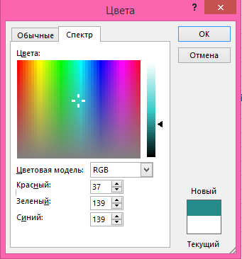
Если вы знаете числовые значения составляющих нужного цвета, в поле Цветовая модель выберите модель RGB (Red, Green, Blue — красный, зеленый, синий) или HSL (Hue, Sat, Lum — тон, насыщенность, яркость), а затем введите числа, в точности соответствующие искомому цвету.
Совет: Чтобы быстро скопировать используемый цвет текста в другие ячейки, выделите исходную ячейку и дважды нажмите кнопку Формат по образцу  . Затем щелкните ячейки, которые нужно отформатировать. По завершении еще раз нажмите кнопку Формат по образцу, чтобы выйти из этого режима.
Форматирование цвета ярлычка листа
Щелкните правой кнопкой мыши ярлычок листа, цвет которого вы хотите изменить.
Щелкните Цвет ярлычка, а затем выберите нужный цвет.
Изменится цвет ярлычка, но не цвет шрифта. При выборе темного цвета ярлычка цвет шрифта меняется на белый, а при выборе светлого цвета — на черный.
Источник
How to change the font color in Excel
Transcript
In this lesson we’ll look at how to change the font color.
Let’s take a look.
Let’s continue with our menu project and add some font colors. Let’s make the headings one color and the menu items another.
Even though we want the headings to be a different color, it will be easiest if we apply one color to the entire worksheet, and then come back and work on the headings separately. As always, start by selecting the cells to format.
The easiest way to apply font color is to use the Font color menu on the home tab of the ribbon. Click once to open the menu, then release the mouse button to browse colors.
This menu shows all of the available colors in the currently selected color scheme. We’ll look at how to change these colors in an upcoming lesson.
To preview a color, just hover over a color square. Excel will show a preview of this color applied. To leave the Font color menu without applying a color, just press the Escape key.
Let’s set the color of all text to a dark gray. Now, let’s try green for the headings.
If the color you’ve selected isn’t quite right, you can easily make adjustments by using the «More Colors» option at the bottom of the Font color menu.
Let’s make the green color darker. Switch from the Standard tab to the Custom tab, and make adjustments as needed. In this case, we can just drag the slider down to get a darker green.
Note that when you’ve customized a color, it will automatically show up in the Font Color menu under Recent Colors. When you want to use a customized color again, you can find it here. Also note that the font color button remembers the last color you used. When you click it again, Excel will apply that color.
Источник
Change the appearance of your worksheet
To change the text fonts, colors, or general look of objects in all worksheets of your workbook quickly, try switching to another theme or customizing a theme to meet your needs. If you like a specific theme, you can make it the default for all new workbooks.
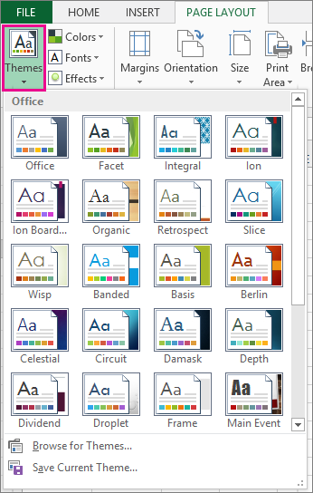
To switch to another theme, click Page Layout > Themes, and pick the one you want.
To customize that theme, you can change its colors, fonts, and effects as needed, save them with the current theme, and make it the default theme for all new workbooks if you want.
Change theme colors
Picking a different theme color palette or changing its colors will affect the available colors in the color picker and the colors you’ve used in your workbook.
Click Page Layout > Colors, and pick the set of colors you want.
The first set of colors is used in the current theme.
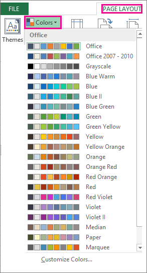
To create your own set of colors, click Customize Colors.
For each theme color you want to change, click the button next to that color, and pick a color under Theme Colors.
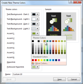
To add your own color, click More Colors, and then pick a color on the Standard tab or enter numbers on the Custom tab.
Tip: In the Sample box, you get a preview of the changes you made.
In the Name box, type a name for the new color set, and click Save.
Tip: You can click Reset before you click Save if you want to return to the original colors.
To save these new theme colors with the current theme, click Page Layout > Themes > Save Current Theme.
Change theme fonts
Picking a different theme font lets you change your text at once. For this to work, make sure Body and Heading fonts are used to format your text.
Click Page Layout > Fonts, and pick the set of fonts you want.
The first set of fonts is used in the current theme.
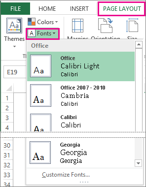
To create you own set of fonts, click Customize Fonts.
In the Create New Theme Fonts box, in the Heading font and Body font boxes, pick the fonts you want.
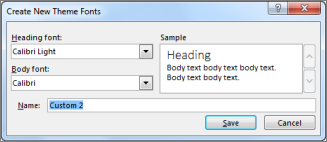
In the Name box, type a name for the new font set, and click Save.
To save these new theme fonts with the current theme, click Page Layout > Themes > Save Current Theme.
Change theme effects
Picking a different set of effects changes the look of the objects you used in your worksheet by applying different types of borders and visual effects like shading and shadows.
Click Page Layout > Effects, and pick the set of effects you want.
The first set of effects is used in the current theme.
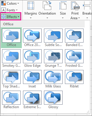
Note: You can’t customize a set of effects.
To save the effects you selected with the current theme, click Page Layout > Themes > Save Current Theme.
Save a custom theme for reuse
After making changes to your theme, you can save it to use it again.
Click Page Layout > Themes > Save Current Theme.
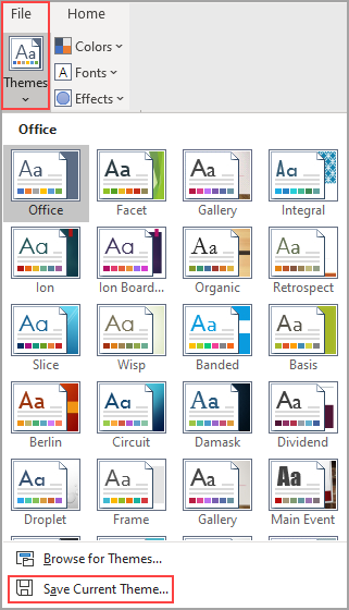
In the File name box, type a name for the theme, and click Save.
Note: The theme is saved as a theme file (.thmx) in the Document Themes folder on your local drive and is automatically added to the list of custom themes that appear when you click Themes.
Use a custom theme as the default for new workbooks
To use your custom theme for all new workbooks, apply it to a blank workbook and then save it as a template named Book.xltx in the XLStart folder (typically C:Users user nameAppDataLocalMicrosoftExcelXLStart).
To set up Excel so it automatically opens a new workbook that uses Book.xltx:
Click File> Options.
On the General tab, under Start up options, uncheck the Show the Start screen when this application starts box.
Источник
Excel Format Fonts
Format Fonts
You can format fonts in four different ways: color, font name, size and other characteristics.
Font Color
The default color for fonts is black.
Colors are applied to fonts by using the «Font color» function.
How to apply colors to fonts
- Select cell
- Select font color
- Type text
The font color goes for both numbers and text.
The Font color command remembers the color used last time.
Note: Custom colors are applied in the same way for both cells and fonts. You can read more about it in the Apply colors to cells chapter.
Lets try an example, step by step:
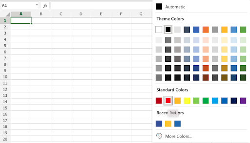
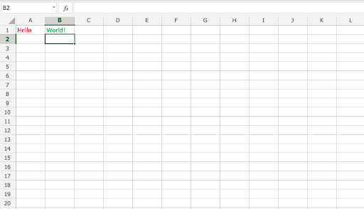
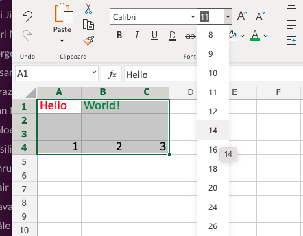
- Select standard font color Red
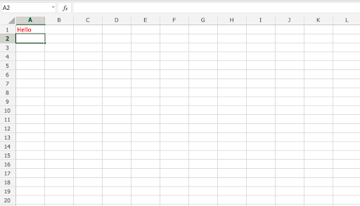
- Type A1(Hello)
- Hit enter
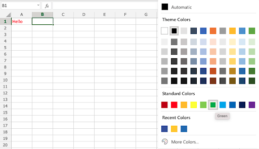
- Select standard font color Green
- Type B1(World!)
- Hit enter
Font Name
The default font in Excel is Calibri.
The font name can be changed for both numbers and text.
Why change the font name in Excel?
- Make the data easier to read
- Make the presentation more appealing
How to change the font name:
- Select a range
- Click the font name drop down menu
- Select a font
Let’s have a look at an example.
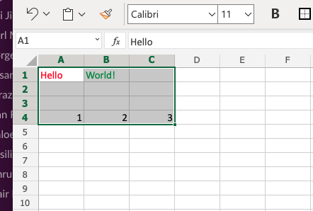
- Select A1:C4
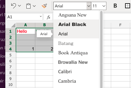
- Click the font name drop down menu
- Select Arial
The example has both text ( A1:B1 ) and numbers ( A4:C4 )
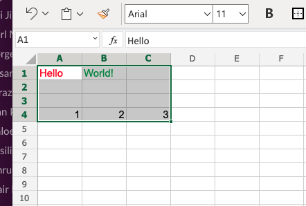
Good job! You have successfully changed the fonts from Calibri to Arial for the range A1:C4 .
Font Size
To change the font size of the font, just click on the font size drop down menu:
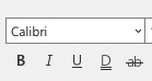
Font Characteristics
You can apply different characteristics to fonts such as:
- Bold
- Italic
- Underlined
- Strike though
The commands can be found below the font name drop down menu:
Bold is applied by either clicking the Bold (B) icon in the Ribbon or using the keyboard shortcut CTRL + B or Command + B
Italic is applied by either clicking the Italic (I) icon or using the keyboard shortcut CTRL + I or Command + I
Underline is applied by either clicking the Underline (U) icon or using the keyboard shortcut CTRL + U or Command + U
Strikethrough is applied by either clicking the Strikethrough (ab) icon or using the keyboard shortcut CTRL + 5 or Command + Shift + X
Chapter Summary
Fonts can be changed in four different ways: color, font name, size and other characteristics. The fonts are changed to make the spreadsheet more readable and delicate.
Источник
Change the color of text
You can make the data on your worksheets more visible by changing the font color of cells or a range of cells, formatting the color of worksheet tabs, or changing the color of formulas.
For information on changing the background color of cells, or applying patterns or fill colors, see Add or change the background color of cells.
Change the text color for a cell or range of cells
Select the cell or range of cells that has the data you want to format. You can also select just a portion of the text within a cell.
On the Home tab, choose the arrow next to Font Color  .
.
Under Theme Colors or Standard Colors, choose a color.
Tip: To apply the most recently selected text color, on the Home tab, choose Font Color.
Apply a custom color
If you want a specific font color, here’s how you can blend your custom color:
Click Home > Font Color arrow > More Colors.
On the Custom tab, in the Colors box, select the color you want.
If you know the color numbers of a specific color, pick RGB (Red, Green, Blue) or HSL (Hue, Sat, Lum) in the Color model box, and then enter the numbers to match the exact color shade you want.
Tip: To quickly copy a font color you used to other cells, select a cell with that font color, and double-click Format Painter . Then click the cells you want to format. When you’re done, click Format Painter again to turn it off.
Format the color of a worksheet tab
Right-click the worksheet tab whose color you want to change.
Choose Tab Color, and then select the color you want.
The color of the tab changes, but not the color of the font. When you choose a dark tab color, the font switches to white, and when you choose a light color for the tab, the font switches to black.
Источник
Format Fonts
You can format fonts in four different ways: color, font name, size and other characteristics.
Font Color
The default color for fonts is black.
Colors are applied to fonts by using the «Font color» function.
How to apply colors to fonts
- Select cell
- Select font color
- Type text
The font color goes for both numbers and text.
The Font color command remembers the color used last time.
Note: Custom colors are applied in the same way for both cells and fonts. You can read more about it in the Apply colors to cells chapter.
Lets try an example, step by step:
- Select standard font color Red
- Type A1(Hello)
- Hit enter
- Select standard font color Green
- Type B1(World!)
- Hit enter
Font Name
The default font in Excel is Calibri.
The font name can be changed for both numbers and text.
Why change the font name in Excel?
- Make the data easier to read
- Make the presentation more appealing
How to change the font name:
- Select a range
- Click the font name drop down menu
- Select a font
Let’s have a look at an example.
- Select
A1:C4 - Click the font name drop down menu
- Select Arial
The example has both text (A1:B1) and numbers (A4:C4)
Good job! You have successfully changed the fonts from Calibri to Arial for the range A1:C4.
Font Size
To change the font size of the font, just click on the font size drop down menu:
Font Characteristics
You can apply different characteristics to fonts such as:
- Bold
- Italic
- Underlined
- Strike though
The commands can be found below the font name drop down menu:
Bold is applied by either clicking the Bold (B) icon in the Ribbon or using the keyboard shortcut CTRL + B or Command + B
Italic is applied by either clicking the Italic (I) icon or using the keyboard shortcut CTRL + I or Command + I
Underline is applied by either clicking the Underline (U) icon or using the keyboard shortcut CTRL + U or Command + U
Strikethrough is applied by either clicking the Strikethrough (ab) icon or using the keyboard shortcut CTRL + 5 or Command + Shift + X
Chapter Summary
Fonts can be changed in four different ways: color, font name, size and other characteristics. The fonts are changed to make the spreadsheet more readable and delicate.

This Excel tutorial explains how to change the font color of a cell in Excel 2016 (with screenshots and step-by-step instructions).
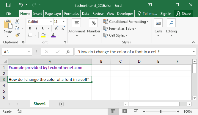
Question: How do I change the color of a font in a cell in Microsoft Excel 2016?
Answer: By default when you create a new workbook in Excel 2016, all cells will be formatted with a black font. You can change the color of the font within any cell.
To change the font color in a cell, select the text that you wish to change the color of. This can either be the entire cell or only a character in the cell.
Select the Home tab in the toolbar at the top of the screen and click on the Font Color button in the Font group.
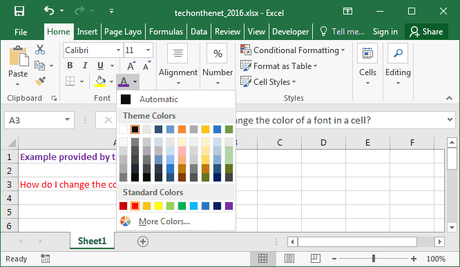
Select the color from the popup window.
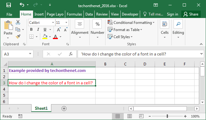
In this example, we’ve chosen to change the font color to red.
Вы когда-нибудь представляли себе это изменение цвета шрифта на основе значения ячейки в Excel? Возьмем, к примеру, когда данные отрицательны, вы можете захотеть, чтобы цвет шрифта данных был красным, или вам нужно, чтобы данные были черными. Здесь я представляю несколько удобных способов, которые помогут вам сэкономить время на изменение цвета шрифта по значению ячейки в Excel.
Изменение цвета шрифта на основе значения ячейки с помощью условного форматирования
Изменить цвет шрифта на основе значения ячейки с помощью параметра «Выбрать определенные ячейки» 
Содержание
- Изменение цвета шрифта на основе значения ячейки с условным форматированием
- Измените цвет шрифта на основе значения ячейки с помощью Select Specific Cells
- Изменить цвет шрифта на основе значения ячейки
- Быстрый подсчет/суммирование ячеек по цвету фона или формата в Excel
Изменение цвета шрифта на основе значения ячейки с условным форматированием
В Excel условное форматирование может помочь при изменении цвета шрифта по ячейке.
(1) Измените цвет шрифта, если он отрицательный/положительный
Если вы хотите изменить цвет шрифта, если значения ячеек отрицательные или положительные, вы можете сделать следующее:
1. Выберите значения ячеек и нажмите Главная > Условное форматирование > Новое правило . См. Снимок экрана:

2. Затем в диалоговом окне Новое правило форматирования выберите Форматировать только ячейки, содержащие в разделе Выбрать тип правила: , и если вы хотите изменить цвет шрифта, если значение ячейки отрицательное, вы можете выбрать Значение ячейки из первого списка и выбрать меньше, чем из среднего списка, и затем введите 0 в правое текстовое поле. См. Снимок экрана:
Совет: Если вы хотите изменить цвет шрифта положительных значений, просто выберите Больше чем из среднего списка.

3. Нажмите Формат , чтобы перейти к диалоговому окну Формат ячеек , затем на вкладке Шрифт выберите нужный цвет из Список цветов . См. Снимок экрана:

4. Нажмите OK > OK , чтобы закрыть диалоговые окна. Теперь все отрицательные значения меняют цвет шрифта на красный.

(2) Изменить цвет шрифта, если больше/меньше чем
Если вы хотите изменить цвет шрифта, когда значения больше или меньше определенного значения , вы можете сделать это следующим образом:
1. Выберите значения ячеек и нажмите Главная > Условное форматирование > Новое правило .
2. Затем в диалоговом окне Новое правило форматирования выберите Форматировать только ячейки, содержащие в разделе Выбрать тип правила: , выберите Значение ячейки из первого списка и больше из среднего списка, а затем введите конкретное значение в правое текстовое поле.. См. Снимок экрана:
Совет: Если вы хотите изменить цвет шрифта, когда значения ячеек меньше определенного значения, просто выберите меньше, чем из среднего списка.

3. Нажмите Формат , чтобы перейти к диалоговому окну Формат ячеек , затем на вкладке Шрифт выберите нужный цвет из Список цветов . Затем нажмите OK > OK , чтобы закрыть диалоговые окна. Все значения больше 50 были изменены на оранжевый цвет шрифта.

(3) Измените цвет шрифта, если он содержит
Если вы хотите изменить цвет шрифта, если значения ячеек содержат определенный текст, например, измените цвет шрифта, если значение ячейки содержит KTE, вы можете сделать следующее:
1. Выберите значения ячеек и нажмите Главная > Условное форматирование > Новое правило .
2. Затем в диалоговом окне Новое правило форматирования выберите Форматировать только ячейки, содержащие в разделе Выбрать тип правила: , выберите Определенный текст из первого списка и Содержит из среднего списка, а затем введите конкретный текст в правое текстовое поле. См. Снимок экрана:

3. Нажмите Формат , чтобы перейти к диалоговому окну Формат ячеек , затем на вкладке Шрифт выберите нужный цвет из Список цветов . Затем нажмите OK > OK , чтобы закрыть диалоговые окна. Все ячейки, содержащие KTE, изменили цвет шрифта на указанный цвет.

Измените цвет шрифта на основе значения ячейки с помощью Select Specific Cells
Если вы хотите попробовать некоторые удобные инструменты надстройки, вы можете попробовать Kutools for Excel , есть утилита под названием Select Specific Cells , которая может быстро выбрать ячейки, соответствующие одному или двум критериям, а затем вы можете изменить цвет шрифта.
| Kutools for Excel , с более чем 300 удобных функций, облегчающих вашу работу. |
|
Бесплатная загрузка |
После бесплатной установки Kutools for Excel, сделайте следующее:
1. Выберите ячейки, с которыми вы хотите работать, и нажмите Kutools > Выбрать > Выбрать определенные ячейки . См. Снимок экрана:

2. В диалоговом окне Выбрать определенные ячейки установите флажок Ячейка в разделе Тип выбора и выберите Содержит в разделе Определенный тип , затем введите конкретный текст в текстовое поле

3. Нажмите Ok > OK , чтобы закрыть диалоговые окна.

4. Затем были выделены все ячейки, содержащие KTE, и перейдите в Home > Font Color , чтобы выбрать нужный цвет шрифта.

Примечание.
1. С помощью Kutools for Excel’s Выбрать определенные ячейки , вы также можете выбрать ячейки, соответствующие нижеприведенному критерию:

2. Также вы можете выбрать ячейки, соответствующие двум критериям. Выберите первый критерий из первого раскрывающегося списка, затем выберите второй критерий из второго раскрывающегося списка, и если вы хотите выбрать ячейки, соответствующие двум критериям одновременно, отметьте опцию И , если вы хотите выбрать ячейки соответствует одному из двух критериев, установите флажок Или .


Щелкните здесь, чтобы узнать больше о выборе конкретных ячеек.
Изменить цвет шрифта на основе значения ячейки
Kutools for Excel: 300+ функций, которые вы должны иметь в Excel, 30-дневная бесплатная пробная версия отсюда.
Быстрый подсчет/суммирование ячеек по цвету фона или формата в Excel |
| В некоторых случаях у вас может быть диапазон ячеек с несколькими цветами, и вы хотите подсчитать/суммировать значения ed на том же цвете, как можно быстро рассчитать? С Kutools for Excel Подсчет по цвету , вы можете быстро выполнить множество вычислений по цвету, а также создать отчет о рассчитанный результат. Нажмите, чтобы получить бесплатную полнофункциональную пробную версию через 30 дней! |
 |
| Kutools для Excel: с более чем 300 удобными надстройками Excel, бесплатная пробная версия без ограничений в течение 30 дней. |
This post will guide you how to change the font color based on cell value in Excel. How do I color cell based on cell value using the conditional formatting feature in Excel.
- Changing Font Color Based on Cell Value
- Video: Changing Font color based on Cell Value
Assuming that you have a list of data in range A1:C6, and you want to change the font color based values in A1:C4 cells, if the value is greater than 5, then changing the font color as red, otherwise, changing the font color as green. To changing the font color based on cell value, you need to do the following steps:
#1 select the range of cells which contain cell values, such as: A1:C6.
#2 go to HOME tab, click Conditional Formatting command under Styles group, and then click New Rule from the drop down men list. And the New Formatting Rule dialog will open.
#3 In New Formatting Rule dialog, select Format only cells that contain in the Select a Rule Type list box, chose Cell Value from the first list box, and select greater than from the second list, type number 5 into last text box under Format only cell with section.
#4 click Format button, and switch to Font tab in Format cells dialog, and choose one color as you need in Color list box. Click OK button.
#5 click Ok button. The Font color has been changed as red if the cell value is greater than 5 in the selected range of cells.
#6 repeat step 3, and create a new rule, select less than from the second list , and type number 5 into last text box under Format only cell with section. And click Format button, choose green color in Color list box. And click OK button.
#7 let’s see the last result:
Video: Changing Font color Based on Cell Value
Change Font Color in Excel VBA
Description:
We usually change the font color if we want to highlight some text. If we want to tell the importance of some data, we highlight the text to get the user attention to a particular range in the worksheet. For examples we can change the font color of highly positive figures in to Green or all negative figures in to red color. So that user can easily notice that and understand the data.
In this topic we will see how change the font color in Excel VBA. Again, we change the font color in excel while generating the reports. We may want to highlight the font in red if the values are negative, in green if the values are positive. Or we may change font colors and sizes for headings. etc…
Change Font Color in Excel VBA – Solution(s):
We can change the font color by using Font.ColorIndex OR Font.Color Properties of a Range/Cell.
Change Font Color in Excel VBA – Examples
The following examples will show you how to change the font color in Excel using VBA.
'In this Example I am changing the Range B4 Font Color
Sub sbChangeFontColor()

'Using Cell Object
Cells(4, 2).Font.ColorIndex = 3 ' 3 indicates Red Color

'Using Range Object
Range("B4").Font.ColorIndex = 3

'--- You can use use RGB, instead of ColorIndex -->
'Using Cell Object
Cells(4, 2).Font.Color = RGB(255, 0, 0)

'Using Range Object
Range("B4").Font.Color = RGB(255, 0, 0)

End Sub
Instructions:
- Open an excel workbook
- Enter some data in Ranges mentioned above
- Press Alt+F11 to open VBA Editor
- Insert a Module for Insert Menu
- Copy the above code and Paste in the code window
- Save the file as macro enabled workbook
- Press F5 to execute itit
Here is an example screen-shot for changing Font Colors:

We can change the font color while working with the reports. But it is good practice to limit to only few colors, instead of using many colors in a single report. In also need to mantian the same color format while delivering the same kind of report next time.
See the following example screen-shot, we are using the same font and background colors for in ranges in the worksheet. It looks good with same king of colors, instead of using multiple colors.

A Powerful & Multi-purpose Templates for project management. Now seamlessly manage your projects, tasks, meetings, presentations, teams, customers, stakeholders and time. This page describes all the amazing new features and options that come with our premium templates.
Save Up to 85% LIMITED TIME OFFER

All-in-One Pack
120+ Project Management Templates
Essential Pack
50+ Project Management Templates
Excel Pack
50+ Excel PM Templates
PowerPoint Pack
50+ Excel PM Templates
MS Word Pack
25+ Word PM Templates
Ultimate Project Management Template
Ultimate Resource Management Template
Project Portfolio Management Templates
Related Posts
-
- Description:
- Change Font Color in Excel VBA – Solution(s):
- Change Font Color in Excel VBA – Examples
VBA Reference
Effortlessly
Manage Your Projects
120+ Project Management Templates
Seamlessly manage your projects with our powerful & multi-purpose templates for project management.
120+ PM Templates Includes:
4 Comments
-
Sitharth
May 6, 2015 at 3:44 PM — ReplyHi,
I can trying the same code .. but i can’t see any changes in Excel sheet… and also Not throw any Error Messge … What can i do for this…?
Thanks advance…… -
Sitharth
May 6, 2015 at 4:00 PM — ReplyNo Problem…. Code is Working Perfectly….
-
masterji
October 19, 2015 at 4:21 PM — ReplyThanks for the good information.
-
Chinchu Joseph
September 6, 2016 at 10:31 AM — Replyi can trying the same code…….but it shows an error is “object varible not set..” what can i do for this..?
Effectively Manage Your
Projects and Resources
ANALYSISTABS.COM provides free and premium project management tools, templates and dashboards for effectively managing the projects and analyzing the data.
We’re a crew of professionals expertise in Excel VBA, Business Analysis, Project Management. We’re Sharing our map to Project success with innovative tools, templates, tutorials and tips.
Project Management
Excel VBA
Download Free Excel 2007, 2010, 2013 Add-in for Creating Innovative Dashboards, Tools for Data Mining, Analysis, Visualization. Learn VBA for MS Excel, Word, PowerPoint, Access, Outlook to develop applications for retail, insurance, banking, finance, telecom, healthcare domains.
Page load link
Go to Top
Transcript
In this lesson we’ll look at how to change the font color.
Let’s take a look.
Let’s continue with our menu project and add some font colors. Let’s make the headings one color and the menu items another.
Even though we want the headings to be a different color, it will be easiest if we apply one color to the entire worksheet, and then come back and work on the headings separately. As always, start by selecting the cells to format.
The easiest way to apply font color is to use the Font color menu on the home tab of the ribbon. Click once to open the menu, then release the mouse button to browse colors.
This menu shows all of the available colors in the currently selected color scheme. We’ll look at how to change these colors in an upcoming lesson.
To preview a color, just hover over a color square. Excel will show a preview of this color applied. To leave the Font color menu without applying a color, just press the Escape key.
Let’s set the color of all text to a dark gray. Now, let’s try green for the headings.
If the color you’ve selected isn’t quite right, you can easily make adjustments by using the «More Colors» option at the bottom of the Font color menu.
Let’s make the green color darker. Switch from the Standard tab to the Custom tab, and make adjustments as needed. In this case, we can just drag the slider down to get a darker green.
Note that when you’ve customized a color, it will automatically show up in the Font Color menu under Recent Colors. When you want to use a customized color again, you can find it here. Also note that the font color button remembers the last color you used. When you click it again, Excel will apply that color.