
Содержание
- Number format codes
- Create a custom format code
- Format code guidelines
- Floating-point number in Excel
- 2 Answers 2
- olpa, OSS developer
- using xlrd and formatting Excel numbers
- The problem for an user
- The problem for a programmer
- The idea
- Usage
- One Response to “using xlrd and formatting Excel numbers”
- Leave a Reply
- Доступные числовые форматы в Excel
- Числовые форматы
- Дополнительные сведения
Number format codes
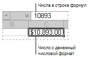
You can use number formats to change the appearance of numbers, including dates and times, without changing the actual number. The number format does not affect the cell value that Excel uses to perform calculations. The actual value is displayed in the formula bar.
Excel provides several built-in number formats. You can use these built-in formats as is, or you can use them as a basis for creating your own custom number formats. When you create custom number formats, you can specify up to four sections of format code. These sections of code define the formats for positive numbers, negative numbers, zero values, and text, in that order. The sections of code must be separated by semicolons (;).
The following example shows the four types of format code sections.

 Format for positive numbers
 Format for negative numbers
 Format for zeros
 Format for text
If you specify only one section of format code, the code in that section is used for all numbers. If you specify two sections of format code, the first section of code is used for positive numbers and zeros, and the second section of code is used for negative numbers. When you skip code sections in your number format, you must include a semicolon for each of the missing sections of code. You can use the ampersand (&) text operator to join, or concatenate, two values.
Create a custom format code
On the Home tab, click Number Format  , and then click More Number Formats.
In the Format Cells dialog box, in the Category box, click Custom.
In the Type list, select the number format that you want to customize.
The number format that you select appears in the Type box at the top of the list.
In the Type box, make the necessary changes to the selected number format.
Format code guidelines
To display both text and numbers in a cell, enclose the text characters in double quotation marks (» «) or precede a single character with a backslash (). Include the characters in the appropriate section of the format codes. For example, you could type the format $0.00″ Surplus»;$–0.00″ Shortage» to display a positive amount as «$125.74 Surplus» and a negative amount as «$–125.74 Shortage.»
You don’t have to use quotation marks to display the characters listed in the following table:
Circumflex accent (caret)
Left curly bracket
Right curly bracket
Greater than sign
To create a number format that includes text that is typed in a cell, insert an «at» sign (@) in the text section of the number format code section at the point where you want the typed text to be displayed in the cell. If the @ character is not included in the text section of the number format, any text that you type in the cell is not displayed; only numbers are displayed. You can also create a number format that combines specific text characters with the text that is typed in the cell. To do this, enter the specific text characters that you want before the @ character, after the @ character, or both. Then, enclose the text characters that you entered in double quotation marks (» «). For example, to include text before the text that’s typed in the cell, enter «gross receipts for «@ in the text section of the number format code.
To create a space that is the width of a character in a number format, insert an underscore (_) followed by the character. For example, if you want positive numbers to line up correctly with negative numbers that are enclosed in parentheses, insert an underscore at the end of the positive number format followed by a right parenthesis character.
To repeat a character in the number format so that the width of the number fills the column, precede the character with an asterisk (*) in the format code. For example, you can type 0*– to include enough dashes after a number to fill the cell, or you can type *0 before any format to include leading zeros.
You can use number format codes to control the display of digits before and after the decimal place. Use the number sign (#) if you want to display only the significant digits in a number. This sign does not allow the display non-significant zeros. Use the numerical character for zero (0) if you want to display non-significant zeros when a number might have fewer digits than have been specified in the format code. Use a question mark (?) if you want to add spaces for non-significant zeros on either side of the decimal point so that the decimal points align when they are formatted with a fixed-width font, such as Courier New. You can also use the question mark (?) to display fractions that have varying numbers of digits in the numerator and denominator.
If a number has more digits to the left of the decimal point than there are placeholders in the format code, the extra digits are displayed in the cell. However, if a number has more digits to the right of the decimal point than there are placeholders in the format code, the number is rounded off to the same number of decimal places as there are placeholders. If the format code contains only number signs (#) to the left of the decimal point, numbers with a value of less than 1 begin with the decimal point, not with a zero followed by a decimal point.
Источник
Floating-point number in Excel
I’ve a little problem with a double value in my excel sheet. The double value is the result of a macro computation. It is displayed into the cell as 1.0554 . The cell format is Number with 4 decimal points displayed. If I choose more decimal, it will be displayed with trailing 0s (E.G. 1.05540000 ).
My problem is I’m reading this file with jxls (which is using Apache POI), and the value I’m getting is not 1.0554 but 1.0554000000000001 (the last 1 is at the 16th digit).
I’ve convert my xls to xlsx, check directly inside the xlsx (which is a zip file containing xml files, so ascii file) and the saved value is 1.0554000000000001 ; but even if I format my cell as a number with 32 decimal, excel still displays 1.0554000. 000 without any trailing 1.
So I suppose that in xls, the real number is also saved as 1.0554000000000001 and not 1.0554.
So how to display in excel the real raw value? or to force excel to save 1.0554 instead of 1.05540000. 01? Or to check with macro that the display value is not the raw value.

2 Answers 2
You have run afoul of the IEE754 gods. Double values have 1 sign bit, 11 bits of exponent and 52 bits of mantissa (the actual representation is a bit more complicated, but what you should take away from this is that the number 1.0554 is not expressible correctly within 52 bits, so the double implementation of your PC chooses the nearest value.

Floating point rounding error comes into play as soon as you convert a number that cannot be represented exactly. It tends to increase as you do calculations.
The closest representable value to 1.0554 is 1.0553999999999998937738610038650222122669219970703125. The closest representable value to 1.0554000000000001 is 1.055400000000000115818465928896330296993255615234375 — that is probably what came out of your macro calculation. The bad news is that you don’t get exactly the value you meant. The good news is that the difference is often, as in this case, far too small to matter, or even be measured, in real life.
Generally, you do not want the exact value printed. The default toString behavior in Java is to produce the shortest decimal expansion that would convert to the internal value. That is also not usually what you want for end-user displays.
The right thing to do, in most cases, is exactly what you are doing in Excel — display only the digits you think matter for what you are doing. In Java, you can use DecimalFormat to convert a double to a String with control over the displayed digits.
Источник
olpa, OSS developer
using xlrd and formatting Excel numbers
The number (and dates) in Excel are float numbers. How these numbers are displyed to an user — as an integer, or with two digits after a point, etc — are defined by the cell format. Unfortunately, xlrd does not support number formatting. It is your task to interpret the format and display the number as expected. My code can probably help. Download xlrd-format-excel-number
The problem for an user
This is how you format a table in Excel:

Let’s dump the the table (see the attached code “dump-sheet.py”):
A naive approach to get a value from a cell is:
“N” can’t be “4.0” or “2.0”, it should be “4” or “2”
Price can’t be “5.0”, it should be “5.00”, or more precisely (in Germany) “5,00”.
The problem for a programmer
The format specification is too hard for a quick implementation:
Nobody has enough time to implement everything.
And there are also border and hidden cases, like this format for currency:
I just have no slightest idea how to get the euro-sign from the format chunk “ [$€-407] “. And there are also conditions. And locale-aware formatting. No, I can’t.
The idea
* Find a substring, which consists of a mix of zeros, hashes, dots and commas.
* Then to use only this substring for further formatting.
It works at least for integer numbers and numbers with two digits after a comma. For my needs, it is 100% of all the use cases. It should work also for many other formats.
If your formats are more complex than the code can handle, you are welcome to extend the code in “numfmt.py”. Don’t forget to add tests into “numfmt_test.py”.
Usage
The example is “dump-sheet.py”. First you have to decide which separators for number part you want to use. A good idea is to get them from the locale user settings.
The sample function format_number takes three parameters:
* f is the float number to format,
* cell and wb are the cell and workbook objects, they are used to find the format string.
The code to get s_fmt (the format string) is found somewhere in the internet, now I can’t remember the source.
The last remark: the call to xlrd.open_workbook should contain the parameter formatting_info=1, otherwise you can’t access the format strings.
Now the python code prints the table correct:
This entry was posted by olpa on Tuesday, October 22nd, 2013 at 9:45 am and is filed under python. You can follow any responses to this entry through the RSS 2.0 feed. You can leave a response, or trackback from your own site.
One Response to “using xlrd and formatting Excel numbers”
The code should be improved. There is a border case: one uses the format “General”. In this case, the “a_fmt” is None, and the string representation is again bad. Solution: after
tail = s_f[-2:]
if (tail == ‘,0’) or (tail == ‘.0’):
s_f = s_f[:-2]
Leave a Reply
olpa, OSS developer is proudly powered by WordPress
Entries (RSS) and Comments (RSS).
Источник
Доступные числовые форматы в Excel
В Excel числа, содержащиеся в ячейках, можно преобразовать, например, в денежные единицы, проценты, десятичные числа, даты, номера телефонов или номера социального страхования США.

Выделите ячейку или диапазон ячеек.
На вкладке Главная выберите в раскрывающемся списке формат Числовой.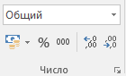
Можно также выбрать один из следующих вариантов:
Нажмите клавиши CTRL+1 и выберите формат Числовой.
Щелкните ячейку или диапазон ячеек правой кнопкой мыши, выберите команду Формат ячеек. и формат Числовой.
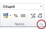
Нажмите небольшую стрелку (кнопку вызова диалогового окна) и выберите Числовой.
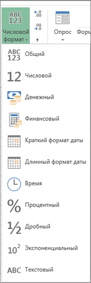
Выберите нужный формат.
Числовые форматы
Чтобы просмотреть все доступные числовые форматы, на вкладке Главная в группе Число нажмите кнопку вызова диалогового окна рядом с надписью Число.
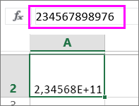
При вводе чисел в Excel этот формат используется по умолчанию. В большинстве случаев числа, имеющие формат Общий, отображаются так, как вводятся. Однако если ширины ячейки недостаточно для отображения всего числа, числа в формате Общий округляются. Для чисел, содержащих более 12 знаков, в формате Общий используется научное (экспоненциальное) представление.
Используется как основной для вывода чисел. Можно задать количество отображаемых знаков после запятой, применение разделителя групп разрядов и способ отображения отрицательных чисел.
Используется для денежных значений и выводит рядом с числом обозначение денежной единицы по умолчанию. Можно задать количество отображаемых знаков после запятой, применение разделителя групп разрядов и способ отображения отрицательных чисел.
Используется для отображения денежных значений с выравниванием обозначений денежных единиц и десятичных разделителей в столбце.
Отображает числовые представления даты и времени как значения даты в соответствии с заданным типом и языковым стандартом (местоположением). Форматы даты, начинающиеся со звездочки ( *), соответствуют формату отображения даты и времени, заданному на панели управления. На форматы без звездочки параметры, заданные на панели управления, не влияют.
Отображает числовые представления даты и времени как значения времени в соответствии с заданным типом и языковым стандартом (местоположением). Форматы времени, начинающиеся со звездочки ( *), соответствуют формату отображения даты и времени, заданному на панели управления. На форматы без звездочки параметры, заданные на панели управления, не влияют.
В этом формате значение ячейки умножается на 100, а результат отображается со знаком процента ( %). Можно задать количество знаков в дробной части.
Отображает число в виде дроби выбранного типа.
Отображает число в экспоненциальном представлении, заменяя часть числа на E+n, где E обозначает экспоненциальное представление, то есть умножение предшествующего числа на 10 в степени n. Например, экспоненциальный формат с двумя знаками в дробной части отображает 12345678901 как 1,23E+10, то есть 1,23, умноженное на 10 в 10-й степени. Можно задать количество знаков в дробной части.
Содержимое ячейки (включая числа) обрабатывается как текст и отображается именно так, как было введено.
Число отображается в виде почтового индекса, телефонного номера или страхового номера (SSN).
Позволяет изменять копию существующего кода числового формата. При этом создается пользовательский числовой формат, добавляемый в список кодов числовых форматов. В зависимости от языковой версии Microsoft Excel можно ввести от 200 до 250 пользовательских числовых форматов. Дополнительные сведения см. в статье Создание и удаление пользовательских числовых форматов.
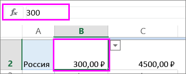
Вы можете применять к числам различные форматы, чтобы изменить способ их отображения. Форматы изменяют только способ отображения чисел и не влияют на значения. Например, если вы хотите, чтобы число отображалось в виде валюты, щелкните ячейку с числом > Денежный.
Форматы влияют только на отображение чисел, но не значения в ячейках, используемые в вычислениях. Фактическое значение можно увидеть в строка формул.
Ниже представлены доступные числовые форматы и описано, как их можно использовать в Excel в Интернете:
Числовой формат по умолчанию. Если ширины ячейки недостаточно, чтобы отобразить число целиком, оно округляется. Например, 25,76 отображается как 26.
Кроме того, если число состоит из 12 или более цифр, при использовании формата Общий значение отображается в экспоненциальном виде.
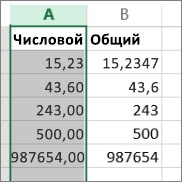
Этот формат похож на Общий, но в отличие от него отображает числа с десятичным разделителем, а также отрицательные числа. Ниже представлено несколько примеров отображения чисел в обоих форматах:
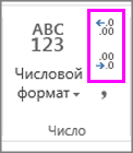
Отображает рядом с числами денежный символ. Чтобы задать необходимое количество знаков после запятой, нажмите кнопку Увеличить разрядность или Уменьшить разрядность.
Используется для отображения денежных значений с выравниванием символов валюты и десятичных разделителей в столбце.
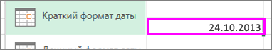
Краткий формат даты
В этом формате дата отображается в следующем виде:
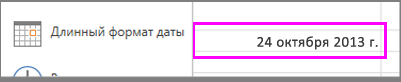
Длинный формат даты
В этом формате месяц, день и год отображаются в следующем виде:
В этом формате числовые представления даты и времени отображаются как значения времени.
В этом формате значение ячейки умножается на 100, а результат отображается со знаком процента ( %).
Чтобы задать необходимое количество знаков после запятой, нажмите кнопку Увеличить разрядность или Уменьшить разрядность.
Отображает число в виде дроби. Например, при вводе 0,5 отображается ½.
Отображает числа в экспоненциальной нотации, заменяя часть числа на E+ n, где E (степень) умножает предыдущее число на 10 в степени n. Например, экспоненциальный формат с двумя знаками в дробной части отображает 12345678901 как 1,23E+10, то есть 1,23, умноженное на 10 в 10-й степени. Чтобы задать необходимое количество знаков после запятой, нажмите кнопку Увеличить разрядность или Уменьшить разрядность.
Содержимое ячейки (включая числа) обрабатывается как текст и отображается именно так, как было введено. Дополнительные сведения о форматировании чисел в виде текста.
Дополнительные сведения
Вы всегда можете задать вопрос специалисту Excel Tech Community или попросить помощи в сообществе Answers community.
Источник
Пользователи Excel часто озадачены очевидной неспособностью Excel выполнять простые математические операции. Это не ошибка программы: компьютеры по своей природе не обладают бесконечной точностью. Excel хранит числа в двоичном формате, используя 8 байт, которых хватает для обработки числа с 15 цифрами.
Некоторые числа не могут быть выражены именно с помощью 8 байт, поэтому хранятся в виде приближений. Чтобы продемонстрировать, как это ограничение может вызывать проблемы, введите следующую формулу в ячейку А1: =(5,1-5,2)+1.
Результат должен быть равен 0,9. Однако если вы отформатируете ячейку так, чтобы она отображала 15 знаков после запятой, то обнаружите, что программа вычисляет формулу с результатом 0,899999999999999 — значением, очень близким к 0,9, но никак не 0,9. Такой результат получается, поскольку операция в круглых скобках выполняется первой, и этот промежуточный результат сохраняется в двоичном формате с использованием приближения. Затем формула добавляет 1 к этому значению, а погрешность приближения распространяется на конечный результат.
Во многих случаях ошибки такого рода не представляют проблемы. Однако если вам необходимо проверить результат формулы с помощью логического оператора, это может стать головной болью. Например, следующая формула (которая предполагает, что предыдущая формула находится в ячейке А1) возвращает ЛОЖЬ: =A1-0,9.
Одно из решений этого типа ошибки заключается в использовании функции ОКРУГЛ. Следующая формула, например, возвращает ИСТИНА, поскольку сравнение выполняется с использованием значения в А1, округленного до одного знака после запятой: =ОКРУГЛ(А1;1)=0.9. Вот еще один пример проблемы точности. Попробуйте ввести следующую формулу: =(1,333-1,233)-(1,334-1,234). Эта формула должна возвращать 0, по вместо этого возвращает -2,22045Е-16 (число, очень близкое к нулю).
Если бы эта формула была в ячейке А1, то формула вернула бы Not Zero: =ЕСЛИ(А1=0;"Zero";"Not Zero"). Один способ справиться с такой ошибкой округления состоит в использовании формулы вроде этой: =ЕСЛИ(ABS(А1)<0.000001;"Zero";"Not Zero"). В данной формуле используется оператор «меньше чем» для сравнения абсолютного значения числа с очень малым числом. Эта формула будет возвращать Zero.
Другой вариант — указать Excel изменить значения листа в соответствии с их отображаемым форматом. Для этого откройте окно Параметры Excel (выберите Файл ► Параметры) и перейдите в раздел Дополнительно. Установите флажок Задать точность как на экране (который находится в области При пересчете этой книги).
Флажок Задать точность как на экране позволяет изменять числа в ваших листах так, что они постоянно будут соответствовать появлению на экране. Этот флажок применяется для всех листов активной книги. Такой вариант не всегда будет вам подходить. Убедитесь, что вы понимаете последствия установки флажка Задать точность как на экране.
Everyone works with floating point numbers daily.
If you go at a supermarket, the prices are like this: 11 eur 29 cents, 23 eur 35 cents and etc. As a C# developer and a blogger, I knew that there is some kind of a problem with the floating points and that the accuracy, but I did not realize how big it was. I thought that it only happens on some floating point numbers or similar.

The truth is unfortunately not a pleasant one – it happens a lot in plenty of calculation with floating points. E.g., if you sum 0,10 with any number above 3, you would definitely not get number + 0,10.
E.g. 10,1-10 is not 0,1!
And that’s enough to say that the calculations are wrong.
Actually, this is not only a bug in Excel, that’s a well-known bug in every computer language, due to the logic of the floating point numbers. In integer representation, every number is represented like the sum of the powers of 2.
E.g., the number 43 is represented as 1+2+8+32. Or (2^0+2^1+2^3+2^5). Not more and not less than exactly 43. What happens, when we want to present decimal numbers? The idea, behind the floating point numbers, is that a floating point numbers are represented like this: 1/2 + 1/4 + 1/8 etc. Thus, the number 0.875 is easily represented as 1/2+1/4+1/8. Or 1/2^1+1/2^2+1/2^3. Quick and simple. And nice.
However, it is really nice to have a number like 0.875, which can be represented easily as sum of 1 divided by some power of 2. But what happens, when we are not that lucky? And we have a number like 0,1? Which is rather often, when we work with decimal? The answer is only one – the computers do not calculate exactly but they give some kind of approximation. And this approximation leads to some interesting facts, that are against mathematics. For example in Excel 12.1-12 is different from 0.1. The reason for this is that 12.1-12 is not 0.1, but 0.99999999999996, because of the problem with the presentation of the floating point numbers. And this is different from 0.1. See the formula yourself:

You may ask yourself, how big is this problem? The answer is – at least as big as infinity. I will confess, I really thought that it does not happen so often, until it happened to me 🙂 Thus, I have made a small research and even built some code to help me calculate ranges of the problem. Here is what the code calculates:

With other words, for every number, between 4 and plus infinity, with a step of 0.1 Excel (and all the computer languages using doubles) makes an error in a simple calculation.
Simple as this one – 5.6-5.5. It is equal to 0.0999999999960 and not 0.1. In the next calculation, 5.7-5.6 we get 0.100000000000001 which is also not 0.1. I have decided to make the code, just to see how many “mistakes” are out there and it turned out that they are really in every number. Check it yourself:
|
1 2 3 4 5 6 7 8 9 10 11 12 13 14 15 16 17 18 19 20 21 22 23 24 25 26 27 28 29 30 31 32 33 34 35 36 37 38 39 40 41 42 43 44 45 46 47 48 49 50 51 52 53 54 55 56 57 58 59 60 61 62 63 64 65 66 67 68 69 70 71 72 73 74 75 76 77 78 79 80 81 82 83 84 85 86 87 88 89 90 91 92 93 94 95 96 97 |
Option Explicit ‘————————————————————————————— ‘ Method : ErrorsNumber ‘ Author : v.doynov ‘ Date : 06.04.2017 ‘ Purpose: Model to see how excel calculates floating point numbers. ‘————————————————————————————— ‘ 0/2 + 0/4 + 0/8 + 1/16 + 1/32 +0/64 + 0/128 + 1/256 + 0/256 +1/512 +0/1024 + 0/2048 ‘ 0,099609375 ‘————————————————————————————— Public Sub ErrorsNumber() Const DIFF_DEFAULT = 0.1 ThisWorkbook.PrecisionAsDisplayed = False Dim lngEndNumber As Long: lngEndNumber = 30 Dim dblStarter As Double Dim dblEnder As Double Dim dblDiff As Double Dim lngCounter As Long Dim lngCounter2 As Long Dim lngRow As Long Dim dblResult As Double Dim lngCountErrors As Long Dim myCell As Range If lngEndNumber > 10000 Then Debug.Print lngEndNumber & «is too big, it takes too much time!»: Exit Sub Call OnStart Cells.Clear For lngCounter = 0 To lngEndNumber dblDiff = DIFF_DEFAULT For lngCounter2 = 0 To 9 dblDiff = DIFF_DEFAULT * lngCounter2 lngRow = lngRow + 1 Set myCell = Cells(lngRow, 1) dblStarter = lngCounter + dblDiff dblEnder = lngCounter + dblDiff + DIFF_DEFAULT dblResult = dblStarter — dblEnder myCell = dblStarter myCell.Offset(0, 1) = dblEnder myCell.Offset(0, 2).FormulaR1C1 = «=RC[-1]-RC[-2]» myCell.Offset(0, 2).NumberFormat = «0.00000000000000000» myCell.Offset(0, 3).FormulaR1C1 = «=IF(RC[-1]=0.1,»«»«,»«X»«)» Next lngCounter2 If lngCounter Mod 100 = 0 Then Debug.Print lngCounter Next lngCounter With Range(«E1») .FormulaR1C1 = «=COUNTIF(C[-1],»«X»«)/» & lngEndNumber * 10 .NumberFormat = «0.0000%» End With Columns.AutoFit Debug.Print «READY!» Call OnEnd End Sub Public Sub OnEnd() Application.ScreenUpdating = True Application.EnableEvents = True Application.AskToUpdateLinks = True Application.DisplayAlerts = True Application.Calculation = xlAutomatic ThisWorkbook.Date1904 = False Application.StatusBar = False End Sub Public Sub OnStart() Application.ScreenUpdating = False Application.EnableEvents = False Application.AskToUpdateLinks = False Application.DisplayAlerts = False Application.Calculation = xlAutomatic ThisWorkbook.Date1904 = False ActiveWindow.View = xlNormalView End Sub |
That’s true, decimals are not exact. And should not be compared.
Anyway, there are always ways to get around this. Excel has introduced the following:
|
ThisWorkbook.PrecisionAsDisplayed = True |
It works quite ok, rounding the numbers to what you see. In C#, we have the decimal variable, which is created exactly to cope up with this problem. And in any other language, we have a work around this. But still, before you see it, you never realize how big this problem is. 🙂 Here is what Microsoft says about the floating-point arithmetics.
Floating point rounding error comes into play as soon as you convert a number that cannot be represented exactly. It tends to increase as you do calculations.
The closest representable value to 1.0554 is 1.0553999999999998937738610038650222122669219970703125. The closest representable value to 1.0554000000000001 is 1.055400000000000115818465928896330296993255615234375 — that is probably what came out of your macro calculation. The bad news is that you don’t get exactly the value you meant. The good news is that the difference is often, as in this case, far too small to matter, or even be measured, in real life.
Generally, you do not want the exact value printed. The default toString behavior in Java is to produce the shortest decimal expansion that would convert to the internal value. That is also not usually what you want for end-user displays.
The right thing to do, in most cases, is exactly what you are doing in Excel — display only the digits you think matter for what you are doing. In Java, you can use DecimalFormat to convert a double to a String with control over the displayed digits.
As one of the most versatile calculators ever created, Excel is utilized to power innumerable business operations daily; however, can it ever fail to give you the correct results?
In the case of floating numbers, it can. The term floating point refers to the fact that there are no constant number of digits before or after the decimal point of a number. In other words, the decimal point itself can “float”.
Calculations may not show the correct results when dealing with high precision values. This is not a bug, but rather a design choice that affects every computing system to some degree.

Binary System
The main reason behind this behavior can be broken down to a fundamental design component of computer-based systems. Computer hardware and software communicate with one another using a binary system, consisting of values 1 and 0, as input and output data.
Therefore, the base-10 numerical system is also stored in binary format, which can cause issues with fractions. For example, the fraction of 2/10 is represented as 0.2 in the decimal number system, but identified by an infinitely repeating number 0.00110011001100110011 in the binary system. Data loss becomes inevitable when storing this number in a finite space. The data loss occurs after the 1E-15 point: more commonly known as the 15-digit limit in Excel.
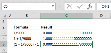
For instance, looking at the example below, you would agree that cells C3 and C5 are equal. However, adding a value of 1 to the value of C3 changes the precision level (i.e. there are eleven 1’s in cell C4, while there are fifteen in cell C3). Ultimately, we get a completely different result in C5, which supposedly contains the inverse function.
Standard
Excel uses a modified version of the IEEE 754-1985 standards. This is a technical standard for floating-point computation, established in 1985 by the Institute of Electrical and Electronics Engineers (IEEE). The 754 revision became very popular and is the most widely used format for floating-point computation by both software libraries and hardware components (i.e. CPUs). According to Microsoft, it is used in all of today’s PC-based microprocessors, including the Intel, Motorola, Sun, and MIPS processors.
Limitations
Maximum / Minimum
Excel only has a finite space to store data. This limitation affects the maximum and minimum numbers allowed by the software. Here are some examples[2]:
| Smallest allowed negative number | -2.2251E-308 |
| Smallest allowed positive number | 2.2251E-308 |
| Largest allowed positive number | 9.99999999999999E+307 |
| Largest allowed negative number | -9.99999999999999E+307 |
| Largest allowed positive number via formula | 1.7976931348623158e+308 |
| Largest allowed negative number via formula | -1.7976931348623158e+308 |
Source: https://support.office.com/en-us/article/excel-specifications-and-limits-1672b34d-7043-467e-8e27-269d656771c3
Excel returns the #NUM! error if a larger number is calculated. This behavior is called an overflow. Excel evaluates very small numbers as 0s, and this behavior is called as underflow. Both will result in data loss.
Excel does not support infinite numbers and provides a #DIV/0! error when a calculation results in an infinite number.
Precision
Although Excel can display more than 15 digits, displayed values are not the actual values that are used in calculations. The IEEE standard upholds storage to only 15 significant digits, which can cause inconsistent results when working with very large or very small numbers.
Very large numbers
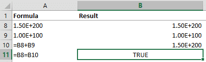
In the example below, Excel finds the sum of B8 and B9 to be equal to the value of B8. The 15-digit limit causes Excel to evaluate the calculation with the 15 largest digits. This example would have required Excel to work with 100-digit precision to evaluate accurately.
Very small numbers
If we add the value 1 to 0.000123456789012345 (which has 18 significant digits but contains numeric values in its smallest 15 digits), the result should be 1.000123456789012345. However, Excel gives 1.00012345678901 because it ignores the digits following the 15th significant digit.

Repeating Binary Numbers
Storing repeating binary numbers as non-repeating decimal number can affect the final values in Excel. For example, the formula ‘=(73.1-73.2)+1’ evaluates to 0.899999999999991 when you format the decimal places to 15 digits.

Accuracy within VBA
Unlike Excel calculations, VBA can work with more than a single type of data. Excel uses 8-byte numbers, while VBA offers different data types that vary from 1 byte (Byte) to 16 bytes (Decimal), which can provide precision at the 28-digit level. You can choose a variable type based on your data storage, accuracy, and speed requirements.
Floating point calculations can be relatively challenging due to technical limitations. However, VBA and other mathematical methods offer workarounds to ensure that you don’t miss a decimal if you’re aware of the existing limitations.