
The Microsoft Excel program is designed not only to enter data into the table conveniently and edit it as you need it, but also to view large blocks of information. Most people using PCs work with it constantly.
The columns and rows names can be significantly removed from the cells with which the user is working at this time. Scrolling the page to see the name of the document is not comfortable for any user. Therefore, the Tabular Processor has possibilities to fix certain areas.
Locking a row in Excel while scrolling
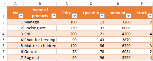
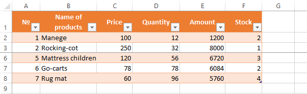
Usually an Excel table has one cap. Meanwhile, this document can have up to thousands of rows. Working with multipage table blocks is inconvenient when column names are not visible. Scrolling the page to its beginning to return to the correct cell is absolutely irrational. To make the cap visible when scrolling, fix the top row of the Excel table, following these actions:
- Create the needed table and fill it with the data.
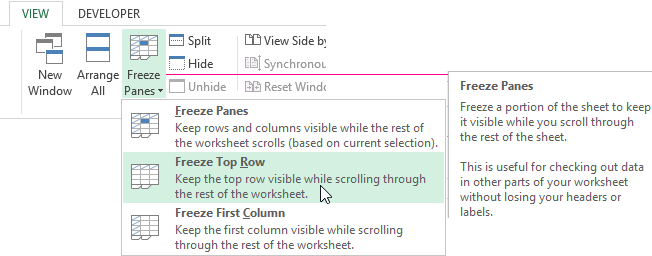
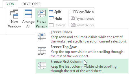
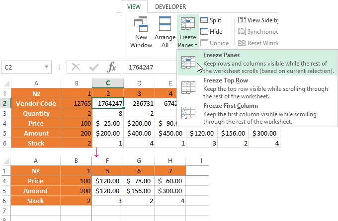
- Make any of the cells active. Go to the “VIEW” tab using the tool “Freeze Panes”.
- In the menu select the “Freeze Top Row” functions.
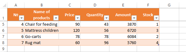
You will get a delimiting line under the top line. Now when you scroll vertically the table cap will be always visible.
Locking several rows in Excel while scrolling
Let us suppose, a user needs to fix not only the cap. For instance, another row or even a couple of rows must be fixed when scrolling the document. Doing it is possible and easy, when you follow these steps:
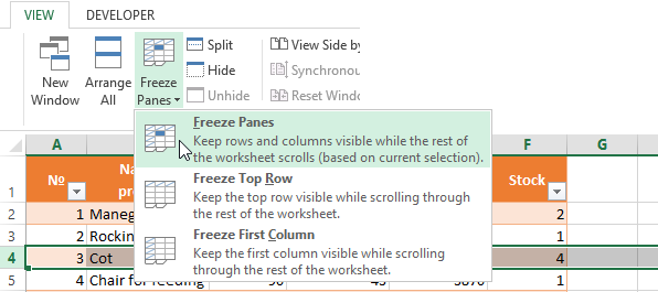
- Select any cell under the line, which we will fix. This action will help Excel to “understand”, which area should be fixed;
- Now select the “Freeze Panes” tool.
When you perform horizontal and vertical scrolling, the cap and the top row of the table remain fixed. Thus, you can fix two, three, four and more rows.
Note: This method works for 2007 and 2010 Excel versions. In earlier versions the “Lock areas” tool is located in the “Window” menu on the main page. There you must always (!) activate the cell under the freeze row.
Freezing columns in Excel
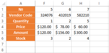
For instance, the information in the table has a horizontal direction. It is not concentrated in columns, but located in rows. For his comfort, the user must freeze the first column, containing the lines’ names in horizontal scrolling.
- Select any cell of the chosen table so that Excel understands with what data it will work. Pin the first column in the menu you will see..
- Now, when the document is scrolled to the right horizontally, the needed column will be fixed.
To freeze several columns, select the cell at the page bottom (to the right from the fixed column). Pick the “Freeze Panes” button.
How to freeze the row and column in Excel
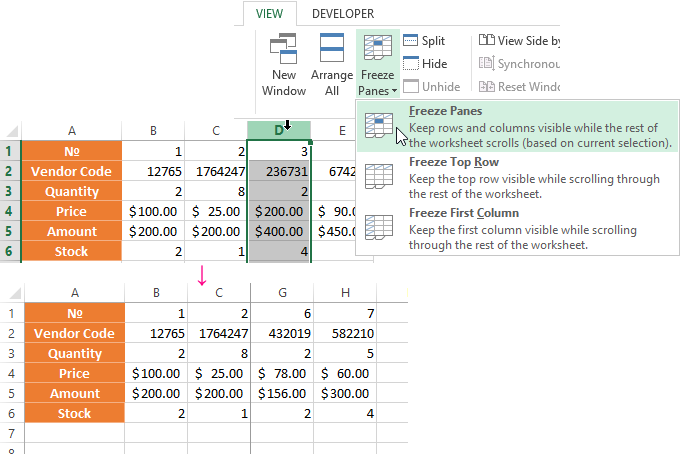
You have a task – to freeze the selected area, which contains two columns and two rows.
Make a cell at the intersection of the fixed rows and columns active. However, the cell must be not placed in the fixed area. It should have the position right under the required lines (to the right of the required columns). Pick the first option in Excel Locking Areas. The photo shows that when scrolling, the selected areas remain at the same place.
Removing a fixed area in Excel
After fixing a row or a column of the table the button deleting all pivot tables becomes available.
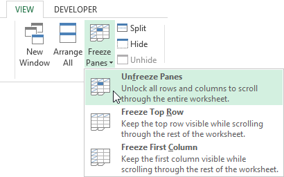
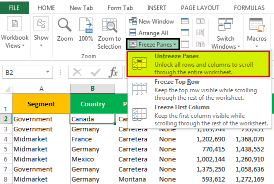
After clicking – «Unfreeze Panes», all the locked areas of the worksheet become unlocked.
Содержание
- Закрепление столбца в таблице Эксель
- Вариант 1: Один столбец
- Вариант 2: Несколько столбцов (область)
- Открепление зафиксированной области
- Заключение
- Вопросы и ответы

В таблицах с большим количеством столбцов довольно неудобно выполнять навигацию по документу, ведь если она в ширину выходит за границы плоскости экрана, для того чтобы посмотреть названия строк, в которые занесены данные, придется постоянно прокручивать страницу влево, а потом опять возвращаться вправо. На эти операции будет уходить дополнительное количество времени. Поэтому для того, чтобы пользователь мог экономить своё время и силы, в программе Microsoft Excel предусмотрена возможность закрепить столбцы. После выполнения данной процедуры левая часть таблицы, в которой находятся наименования строк, всегда будет на виду. Давайте же разберемся, как зафиксировать столбцы в приложении Excel.
Закрепление столбца в таблице Эксель
При работе с «широкой» таблицей может потребоваться закрепить как один, так и сразу несколько столбцов (область). Делается это буквально в несколько кликов, а непосредственный алгоритм выполнения в каждом из двух случаев отличается буквально на один пункт.
Вариант 1: Один столбец
Для того чтобы закрепить крайний левый столбец, можно даже не выделять его предварительно – программа сама поймет, для какого элемента таблицы требуется принять указанное вами изменение.
- Перейдите во вкладку «Вид».
- Разверните меню пункта «Закрепить области».
- Выберите последний вариант в списке доступных опций – «Закрепить первый столбец».
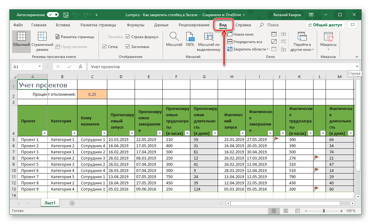

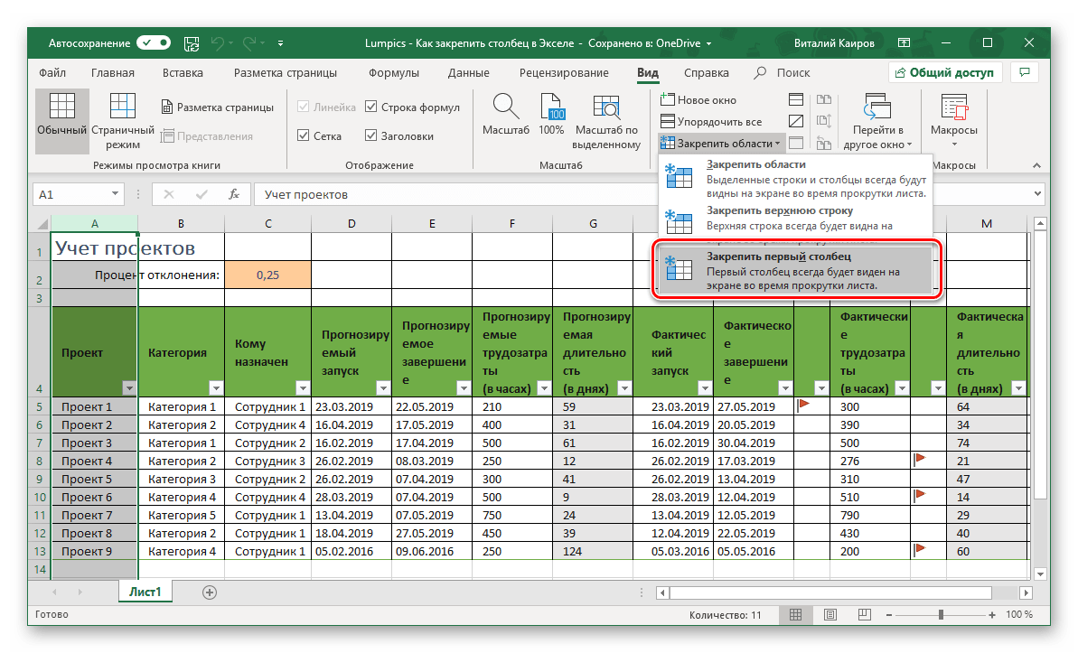
С этого момента при горизонтальной прокрутке таблицы ее первый (левый) столбец всегда будет оставаться на фиксированном месте.
Вариант 2: Несколько столбцов (область)
Бывает и так, что закрепить требуется более одного столбца, то есть область таковых. В данном случае необходимо учесть всего один важный нюанс – не выделяйте диапазон столбцов.
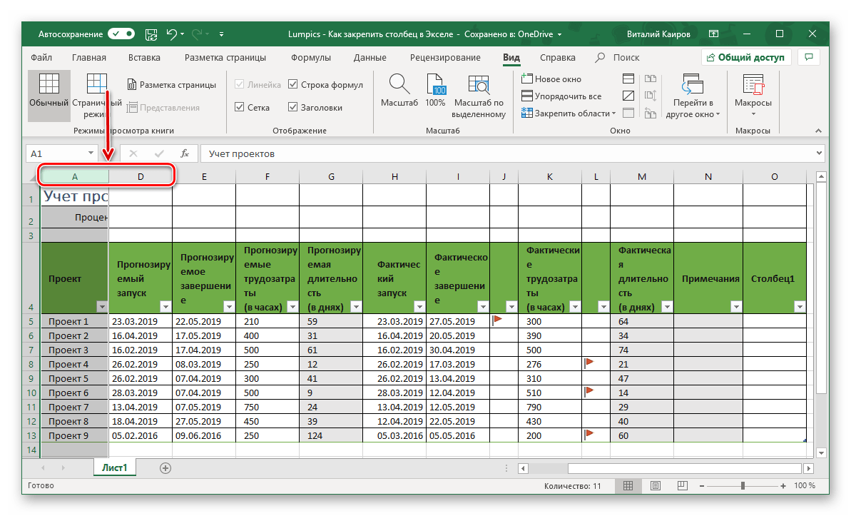
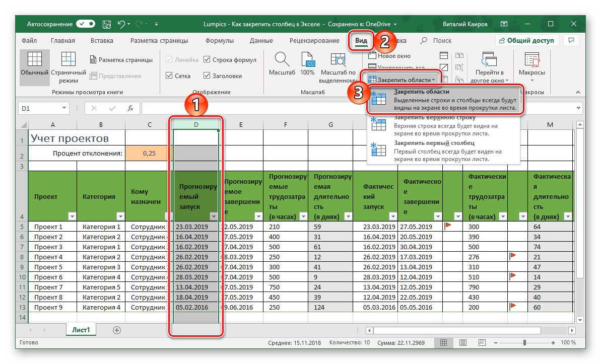
- Выделите столбец, следующий за той областью, которую планируете закрепить. То есть, если требуется закрепить диапазон A-C, выделять необходимо D.
- Перейдите во вкладку «Вид».
- Кликните по меню «Закрепить области» и выберите в нем аналогичный пункт.
Теперь необходимое вам количество столбцов закреплено и при прокрутке таблицы они будут оставаться на своем месте – слева.

Читайте также: Как в Microsoft Excel закрепить область
Открепление зафиксированной области
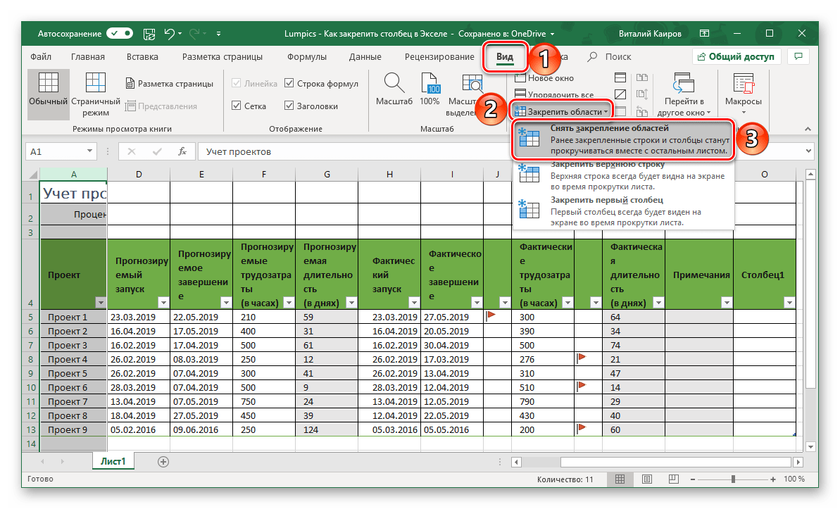
Если необходимость в закреплении столбца или столбцов отпала, во все той же вкладке «Вид» программы Эксель откройте меню кнопки «Закрепить области» и выберите вариант «Снять закрепление областей». Это сработает как для одного элемента, так и для диапазона таковых.
Заключение
Как видите, в табличном процессоре Microsoft Excel можно легко закрепить всего один, крайний левый столбец или диапазон таковых (область). Открепить их, если такая необходимость появится, тоже можно буквально в три клика.
Еще статьи по данной теме:
Помогла ли Вам статья?
Содержание
- Freeze panes to lock rows and columns
- Freeze rows or columns
- Unfreeze rows or columns
- Need more help?
- Resize a table, column, or row
- In this article
- Change column width
- Change row height
- Make multiple columns or rows the same size
- Resize a column or table automatically with AutoFit
- Turn off AutoFit
- Resize an entire table manually
- Add or change the space inside the table
- Freeze Columns in Excel
- #1 Freeze the First Column in Excel
- Example #1
- #2 Freeze Multiple Columns in Excel
- Example #2
- #3 Freeze the Row and Column Together in Excel
- Example #3
- #4 Unfreeze Panes in Excel
- The Rules of Freezing in Excel
- Frequently Asked Questions
- Recommended Articles
Freeze panes to lock rows and columns
To keep an area of a worksheet visible while you scroll to another area of the worksheet, go to the View tab, where you can Freeze Panes to lock specific rows and columns in place, or you can Split panes to create separate windows of the same worksheet.

Freeze rows or columns
Freeze the first column
Select View > Freeze Panes > Freeze First Column.
The faint line that appears between Column A and B shows that the first column is frozen.
Freeze the first two columns
Select the third column.
Select View > Freeze Panes > Freeze Panes.
Freeze columns and rows
Select the cell below the rows and to the right of the columns you want to keep visible when you scroll.
Select View > Freeze Panes > Freeze Panes.
Unfreeze rows or columns
On the View tab > Window > Unfreeze Panes.

Note: If you don’t see the View tab, it’s likely that you are using Excel Starter. Not all features are supported in Excel Starter.
Need more help?
You can always ask an expert in the Excel Tech Community or get support in the Answers community.
Источник
Resize a table, column, or row
Adjust the table size, column width, or row height manually or automatically. You can change the size of multiple columns or rows and modify the space between cells. If you need to add a table to your Word document, see Insert a table.
In this article
Change column width
To change the column width, do one of the following:
To use your mouse, rest the cursor on right side of the column boundary you want to move until it becomes a resize cursor  , and then drag the boundary until the column is the width you want.
To change the width to a specific measurement, click a cell in the column that you want to resize. On the Layout tab, in the Cell Size group, click in the Table Column Width box, and then specify the options you want.
To make the columns in a table automatically fit the contents, click on your table. On the Layout tab, in the Cell Size group, click AutoFit, and then click AutoFit Contents.
To use the ruler, select a cell in the table, and then drag the markers on the ruler. If you want to see the exact measurement of the column on the ruler, hold down ALT as you drag the marker.
Change row height
To change the row height, do one of the following:
To use your mouse, rest the pointer on the row boundary you want to move until it becomes a resize pointer  , and then drag the boundary.
To set the row height to a specific measurement, click a cell in the row that you want to resize. On the Layout tab, in the Cell Size group, click in the Table Row Height box, and then specify the height you want.
To use the ruler, select a cell in the table, and then drag the markers on the ruler. If you want to see the exact measurement of row on the ruler, hold down ALT as you drag the marker.
Make multiple columns or rows the same size
Select the columns or rows you want to make the same size. You can press CTRL while you select to choose several sections that are not next to each other.
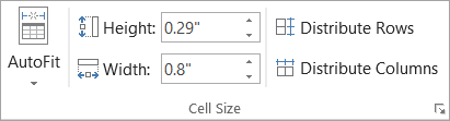
On the Layout tab, in the Cell Size group, click Distribute Columns  or Distribute Rows
  .
.
The entire table
Rest the pointer over the table until the table move handle  appears, and then click the table move handle.
Click to the left of the row. 
A column or columns
Click the column’s top gridline or border. 
Click the left edge of the cell. 
Resize a column or table automatically with AutoFit
Automatically adjust your table or columns to fit the size of your content by using the AutoFit button.
Select your table.
On the Layout tab, in the Cell Size group, click AutoFit.
Do one of the following.
To adjust column width automatically, click AutoFit Contents.
To adjust table width automatically, click AutoFit Window.
Note: Row height automatically adjusts to the size of the content until you manually change it.
Turn off AutoFit
If you don’t want AutoFit to automatically adjust your table or column width, you can turn it off.
Select your table.
On the Layout tab, in the Cell Size group, click AutoFit.
Click Fixed Column Width.
Resize an entire table manually
Rest the cursor on the table until the table resize handle  appears at the lower-right corner of the table.
Rest the cursor on the table resize handle until it becomes a double-headed arrow  .
.
Drag the table boundary until the table is the size you want.
Add or change the space inside the table
To add space inside your table, you can adjust cell margins or cell spacing.
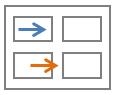
Cell margins are inside the table cell, like the blue arrow on the top of the graphic. Cell spacing is between the cells, like the orange arrow on the bottom.
Click the table.
On the Layout tab, in the Alignment group, click Cell Margins, and then in the Table Options dialog box
Do one of the following:
Under Default cell margins, enter the measurement you want to adjust the Top, Bottom, Left, or Right margins.
Under Default cell spacing, select the Allow spacing between cells check box, and then enter the measurement you want.
Note: The settings that you choose are available only in the active table. Any new tables that you create will use the original default setting.
Источник
Freeze Columns in Excel


Freezing columns in excel fixes or locks them so that they remain visible while scrolling through the database. A frozen column does not move with the movement of the remaining columns.
For example, freezing the first column (column A) ensures that it stays at its place at the time of navigation through the rest of the columns. Moreover, if column A consists of headings, the user may want to view these while working on the other columns of the dataset.
The objectives of freezing an excel column are:
- To ensure that the user does not lose track of the specific column
- To facilitate comparison of different columns of the worksheet
Freezing columns prevents the user from referring to the same column again and again. In other words, the frozen columns save the scrolling time of the user.
All the properties of the frozen column apply to the frozen row as well.
- Freeze panes–It freezes multiple rows and columns.
- Freeze top row–It freezes only the first row.
- Freeze first column–It freezes only the first column.
After freezing a row or column in excel, a grey line appears at the end of the frozen area. This line indicates that the row or column has been frozen.
Table of contents
Let us go through the ways of freezing the first excel column, multiple columns, and both rows and columns.
#1 Freeze the First Column in Excel
Freezing the first column locks column A of the worksheet. This means that on moving from left to right, this column will be visible at all times.
In addition, column A is fixed irrespective of the column from which the actual data begins. The excel shortcut to freeze the first column is “Alt+W+F+C” (when pressed one by one).

Let us consider an example.
Example #1
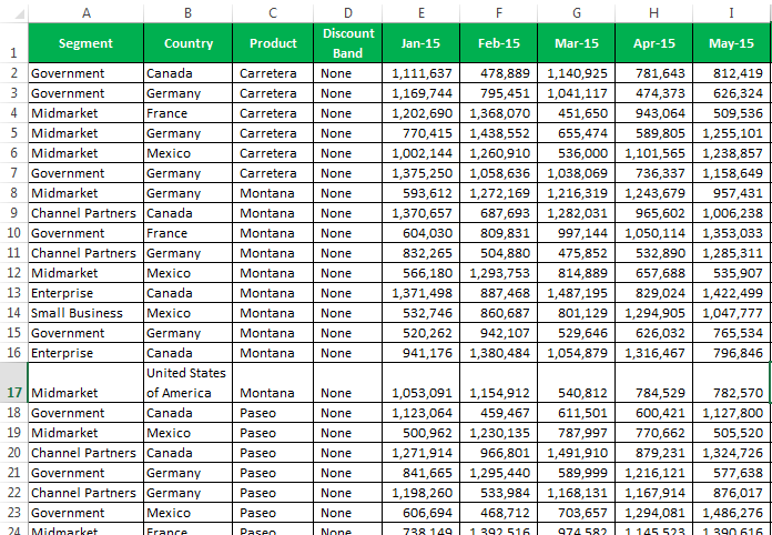
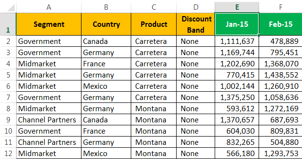
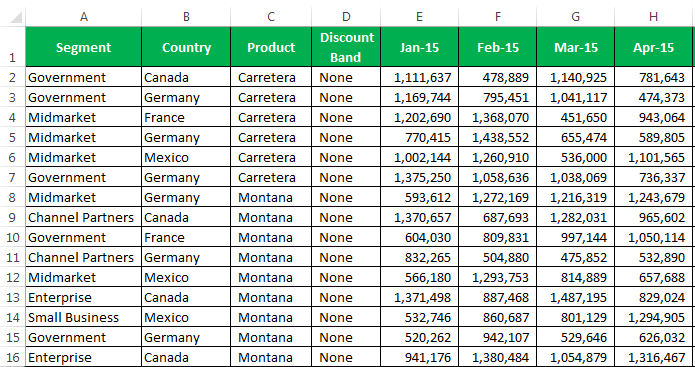
The following table shows the sales revenue (in $) generated by the products of specific segments. The data relates to various countries and is spread across the first five months of the year 2015.
We want to freeze the first excel column (column A).
In order to view the column “segment” on a movement from left to right, we need to freeze it.
The steps for freezing the excel column are listed as follows:
- Select the worksheet where the first column is to be frozen.
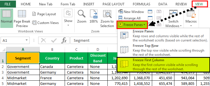
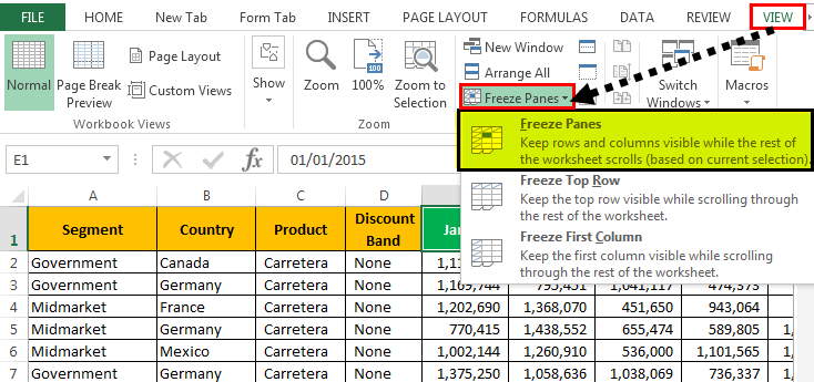
In the View tab, click the “freeze panes” drop-down under the “window” section. Select “freeze first column,” as shown in the succeeding image.
Alternatively, press the shortcut keys “Alt+W+F+C” one by one.
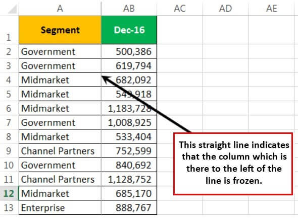
The first column is frozen. The grey line appears at the end of column A indicating that the column to the left is frozen. The column AB shown in the following image is the last scrolled column of the dataset.
On scrolling (from left to right) through the remaining columns of the dataset, column A is visible. The same is shown in the following image.
In the same way, the first row can be frozen.
#2 Freeze Multiple Columns in Excel
Freezing multiple excel columns is similar to freezing multiple rows. For freezing multiple columns, select the first right-hand side cell immediately after the last column to be frozen. This is because multiple columns are frozen based on the current selection.
Similarly, for freezing multiple rows, select the first cell immediately below the last row to be frozen.
For example, to freeze the columns A, B, and C, select the cell D1. By freezing the first three columns, they remain visible to the user at all times. Likewise, to freeze the rows 1, 2, and 3, select the cell A4.
The shortcut to freeze multiple excel columns is “Alt+W+F+F” (when pressed one by one).

Let us consider an example.
Example #2
Working on the data of example #1, we want to freeze the first four columns, A, B, C, and D.
The steps for freezing multiple excel columns are listed as follows:
Step 1: Select the cell E1. This is because the first four columns are to be frozen.
Step 2: In the View tab, click the “freeze panes” drop-down under the “window” section. Select “freeze panes,” as shown in the succeeding image.
Alternatively, press the shortcut keys “Alt+W+F+F” one by one.
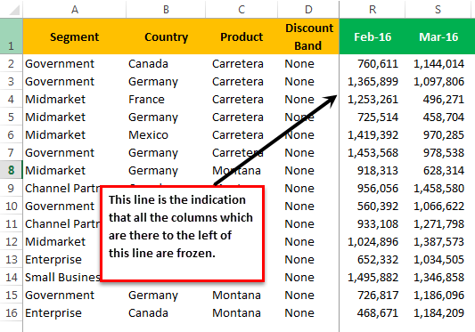
Step 3: The first four columns are frozen. The grey line appears (shown in the following image) at the end of column D, indicating that the columns to the left are frozen.
The columns R and S shown in the following image are the scrolled columns towards the end of the dataset.
Step 4: On scrolling (from left to right) till the last column of the dataset, the first four columns are visible. The same is shown in the following image.
#3 Freeze the Row and Column Together in Excel
Usually, the first row and the first column of a database contain headers. The user might want to view the row 1 and the column A simultaneously and at all times. Hence, it is essential to lock them together to permit their visibility while scrolling down and from left to right.
The only difference between the methods #2 and #3 is in the selection of the cell (step 1). With the “freeze panes” option, Excel freezes the rows and columns preceding the current active cell.
The shortcut to freeze the row and column together is “Alt+W+F+F” (when pressed one by one).
Let us consider an example.
Example #3
Working on the data of example #1, we want to freeze the first row (row 1) and the first column (column A) at the same time.
The steps to freeze the excel row 1 and column A together are listed as follows:
Step 1: Select the cell B2.
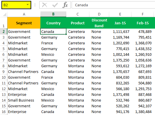
Step 2: Press the shortcut keys “Alt+W+F+F” one by one. It freezes the column to the left of the selected cell B2. At the same time, the row preceding the active cell (B2) is also frozen, as shown in the following image.
Hence two grey lines appear, one at the end of row 1 (horizontal) and the other at the end of column A (vertical).
Note: Alternatively, the “freeze panes” option can be selected from the “freeze panes” drop-down of the View tab.
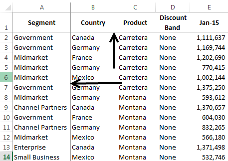
Step 3: On scrolling from top to bottom and left to right, the row 1 and column A are visible. The same is shown in the following image.
Note: It is possible to freeze as many rows and columns depending on the requirement. The condition is that freezing of multiple excel rows and columns should begin with the top row (row 1) and the first column (column A).
#4 Unfreeze Panes in Excel
Unfreezing of panes does not require any cells to be selected. The steps to unfreeze panes in Excel are listed as follows:
Step 1: In the View tab, click the “freeze panes” drop-down under the “window” section. Select “unfreeze panes,” as shown in the succeeding image.
Alternatively, press the shortcut keys “Alt+W+F+F” one by one.
Step 2: The grey lines are removed, as shown in the following image.
Note: The “unfreeze panes” option appears only after freezes have been applied to the Excel worksheet.
The Rules of Freezing in Excel
The norms governing the freezing of rows and columns are listed as follows:
- It is not possible to freeze excel rows and columns in the middle of the worksheet.
- The option “freeze panes” can be applied only once. It is not possible to create multiple “freeze panes” in a single worksheet.
- The rows and columns to be fixed should be visible at the time of freezing. Otherwise, they will remain hidden even after freezing.
Note 1: To divide a worksheet into two or more areas with separate scroll bars Scroll Bars In Excel, there are two scroll bars: one is a vertical scroll bar that is used to view data from up and down, and the other is a horizontal scroll bar that is used to view data from left to right. read more for each, use the “split” option. This is available in the “window” section of the View tab.
Note 2: To fix the header row of a large dataset that does not fit into the screen, create an Excel table Excel Table In excel, tables are a range with data in rows and columns, and they expand when new data is inserted in the range in any new row or column in the table. To use a table, click on the table and select the data range. read more . Moreover, ensure the visibility of this row by selecting any cell within the table before scrolling.
Frequently Asked Questions
Freezing a column means locking it in order to keep it visible while the user scrolls through the database. This is specifically helpful if a column contains headers which are required to be seen at all times.
After freezing, a grey line appears to indicate the frozen columns on its left. The steps to freeze the first column (column A) are listed as follows:
• In the View tab, click the “freeze panes” drop-down under the “window” section.
• Select “freeze first column.” Alternatively, press the shortcut keys “Alt+W+F+C” one by one.
• The first column (column A) is frozen.
Note: For freezing the first row, select “freeze top row” from the “freeze panes” drop-down of the View tab.
Let us freeze columns A, B, C, D, and E. The steps to freeze multiple columns in Excel are listed as follows:
• Select either the column or the first cell to the right of the last column to be frozen (column E). So, select either column F or the cell F1.
• In the View tab, click the “freeze panes” drop-down under the “window” section.
• Select “freeze panes.” Alternatively, press the shortcut keys “Alt+W+F+F” one by one.
• The columns A B, C, D, and E are frozen as indicated by the grey line at the end of column E.
Let us freeze rows 1, 2, and 3 and columns A, B, and C. The steps to freeze the given rows and columns together are listed as follows:
• Select cell D4 based on the following parameters:
a. It immediately follows the last row to be frozen (row 3).
b. It is to the right of the last column to be frozen (column C).
• In the View tab, click the “freeze panes” drop-down under the “window” section.
• Select “freeze panes.” Alternatively, press the shortcut keys “Alt+W+F+F” one by one.
• The rows 1, 2, and 3 and columns A, B, and C are frozen. This is indicated by the grey line appearing below row 3 and at the end of column C.
Note: The freezing of multiple excel rows and columns should begin with the top row (row 1) and the first column (column A).
Recommended Articles
This has been a guide to freezing columns in Excel. Here we discuss how to freeze the first column, multiple columns, and both rows and columns. For more on Excel, take a look at the following articles-
Источник
Freeze panes to lock rows and columns
To keep an area of a worksheet visible while you scroll to another area of the worksheet, go to the View tab, where you can Freeze Panes to lock specific rows and columns in place, or you can Split panes to create separate windows of the same worksheet.
Freeze rows or columns
Freeze the first column
-
Select View > Freeze Panes > Freeze First Column.
The faint line that appears between Column A and B shows that the first column is frozen.
Freeze the first two columns
-
Select the third column.
-
Select View > Freeze Panes > Freeze Panes.
Freeze columns and rows
-
Select the cell below the rows and to the right of the columns you want to keep visible when you scroll.
-
Select View > Freeze Panes > Freeze Panes.
Unfreeze rows or columns
-
On the View tab > Window > Unfreeze Panes.

Note: If you don’t see the View tab, it’s likely that you are using Excel Starter. Not all features are supported in Excel Starter.
Need more help?
You can always ask an expert in the Excel Tech Community or get support in the Answers community.
See Also
Freeze panes to lock the first row or column in Excel 2016 for Mac
Split panes to lock rows or columns in separate worksheet areas
Overview of formulas in Excel
How to avoid broken formulas
Find and correct errors in formulas
Keyboard shortcuts in Excel
Excel functions (alphabetical)
Excel functions (by category)
Need more help?
Want more options?
Explore subscription benefits, browse training courses, learn how to secure your device, and more.
Communities help you ask and answer questions, give feedback, and hear from experts with rich knowledge.
Freezing columns in excel fixes or locks them so that they remain visible while scrolling through the database. A frozen column does not move with the movement of the remaining columns.
For example, freezing the first column (column A) ensures that it stays at its place at the time of navigation through the rest of the columns. Moreover, if column A consists of headings, the user may want to view these while working on the other columns of the dataset.
The objectives of freezing an excel column are:
- To ensure that the user does not lose track of the specific column
- To facilitate comparison of different columns of the worksheet
Freezing columns prevents the user from referring to the same column again and again. In other words, the frozen columns save the scrolling time of the user.
All the properties of the frozen column apply to the frozen row as well.
The “freeze panesFreezing panes in excel helps freeze one or more rows and/or columns so that they remain fixed while scrolling through the database.read more” drop-down under the View tab lists the following options:
- Freeze panes–It freezes multiple rows and columns.
- Freeze top row–It freezes only the first row.
- Freeze first column–It freezes only the first column.
After freezing a row or column in excel, a grey line appears at the end of the frozen area. This line indicates that the row or column has been frozen.
Table of contents
- #1 Freeze the First Column in Excel
- Example #1
- #2 Freeze Multiple Columns in Excel
- Example #2
- #3 Freeze the Row and Column Together in Excel
- Example #3
- #4 Unfreeze Panes in Excel
- The Rules of Freezing in Excel
- Frequently Asked Questions
- Recommended Articles
Let us go through the ways of freezing the first excel column, multiple columns, and both rows and columns.
#1 Freeze the First Column in Excel
Freezing the first column locks column A of the worksheet. This means that on moving from left to right, this column will be visible at all times.
In addition, column A is fixed irrespective of the column from which the actual data begins. The excel shortcut to freeze the first column is “Alt+W+F+C” (when pressed one by one).
Let us consider an example.
Example #1
The following table shows the sales revenue (in $) generated by the products of specific segments. The data relates to various countries and is spread across the first five months of the year 2015.
We want to freeze the first excel column (column A).
In order to view the column “segment” on a movement from left to right, we need to freeze it.
The steps for freezing the excel column are listed as follows:
- Select the worksheet where the first column is to be frozen.
- In the View tab, click the “freeze panes” drop-down under the “window” section. Select “freeze first column,” as shown in the succeeding image.
Alternatively, press the shortcut keys “Alt+W+F+C” one by one.

- The first column is frozen. The grey line appears at the end of column A indicating that the column to the left is frozen. The column AB shown in the following image is the last scrolled column of the dataset.

- On scrolling (from left to right) through the remaining columns of the dataset, column A is visible. The same is shown in the following image.

In the same way, the first row can be frozen.
#2 Freeze Multiple Columns in Excel
Freezing multiple excel columns is similar to freezing multiple rows. For freezing multiple columns, select the first right-hand side cell immediately after the last column to be frozen. This is because multiple columns are frozen based on the current selection.
Similarly, for freezing multiple rows, select the first cell immediately below the last row to be frozen.
For example, to freeze the columns A, B, and C, select the cell D1. By freezing the first three columns, they remain visible to the user at all times. Likewise, to freeze the rows 1, 2, and 3, select the cell A4.
The shortcut to freeze multiple excel columns is “Alt+W+F+F” (when pressed one by one).
Let us consider an example.
Example #2
Working on the data of example #1, we want to freeze the first four columns, A, B, C, and D.
The steps for freezing multiple excel columns are listed as follows:
Step 1: Select the cell E1. This is because the first four columns are to be frozen.
Step 2: In the View tab, click the “freeze panes” drop-down under the “window” section. Select “freeze panes,” as shown in the succeeding image.
Alternatively, press the shortcut keys “Alt+W+F+F” one by one.
Step 3: The first four columns are frozen. The grey line appears (shown in the following image) at the end of column D, indicating that the columns to the left are frozen.
The columns R and S shown in the following image are the scrolled columns towards the end of the dataset.
Step 4: On scrolling (from left to right) till the last column of the dataset, the first four columns are visible. The same is shown in the following image.
#3 Freeze the Row and Column Together in Excel
Usually, the first row and the first column of a database contain headers. The user might want to view the row 1 and the column A simultaneously and at all times. Hence, it is essential to lock them together to permit their visibility while scrolling down and from left to right.
The only difference between the methods #2 and #3 is in the selection of the cell (step 1). With the “freeze panes” option, Excel freezes the rows and columns preceding the current active cell.
The shortcut to freeze the row and column together is “Alt+W+F+F” (when pressed one by one).
Let us consider an example.
Example #3
Working on the data of example #1, we want to freeze the first row (row 1) and the first column (column A) at the same time.
The steps to freeze the excel row 1 and column A together are listed as follows:
Step 1: Select the cell B2.
Step 2: Press the shortcut keys “Alt+W+F+F” one by one. It freezes the column to the left of the selected cell B2. At the same time, the row preceding the active cell (B2) is also frozen, as shown in the following image.
Hence two grey lines appear, one at the end of row 1 (horizontal) and the other at the end of column A (vertical).
Note: Alternatively, the “freeze panes” option can be selected from the “freeze panes” drop-down of the View tab.
Step 3: On scrolling from top to bottom and left to right, the row 1 and column A are visible. The same is shown in the following image.
Note: It is possible to freeze as many rows and columns depending on the requirement. The condition is that freezing of multiple excel rows and columns should begin with the top row (row 1) and the first column (column A).
#4 Unfreeze Panes in Excel
Unfreezing of panes does not require any cells to be selected. The steps to unfreeze panes in Excel are listed as follows:
Step 1: In the View tab, click the “freeze panes” drop-down under the “window” section. Select “unfreeze panes,” as shown in the succeeding image.
Alternatively, press the shortcut keys “Alt+W+F+F” one by one.
Step 2: The grey lines are removed, as shown in the following image.
Note: The “unfreeze panes” option appears only after freezes have been applied to the Excel worksheet.
The Rules of Freezing in Excel
The norms governing the freezing of rows and columns are listed as follows:
- It is not possible to freeze excel rows and columns in the middle of the worksheet.
- The option “freeze panes” can be applied only once. It is not possible to create multiple “freeze panes” in a single worksheet.
- The rows and columns to be fixed should be visible at the time of freezing. Otherwise, they will remain hidden even after freezing.
Note 1: To divide a worksheet into two or more areas with separate scroll barsIn Excel, there are two scroll bars: one is a vertical scroll bar that is used to view data from up and down, and the other is a horizontal scroll bar that is used to view data from left to right.read more for each, use the “split” option. This is available in the “window” section of the View tab.
Note 2: To fix the header row of a large dataset that does not fit into the screen, create an Excel tableIn excel, tables are a range with data in rows and columns, and they expand when new data is inserted in the range in any new row or column in the table. To use a table, click on the table and select the data range.read more. Moreover, ensure the visibility of this row by selecting any cell within the table before scrolling.
Frequently Asked Questions
1. What does freezing columns mean and how to freeze the first column in Excel?
Freezing a column means locking it in order to keep it visible while the user scrolls through the database. This is specifically helpful if a column contains headers which are required to be seen at all times.
After freezing, a grey line appears to indicate the frozen columns on its left. The steps to freeze the first column (column A) are listed as follows:
• In the View tab, click the “freeze panes” drop-down under the “window” section.
• Select “freeze first column.” Alternatively, press the shortcut keys “Alt+W+F+C” one by one.
• The first column (column A) is frozen.
Note: For freezing the first row, select “freeze top row” from the “freeze panes” drop-down of the View tab.
2. How to freeze multiple columns in Excel?
Let us freeze columns A, B, C, D, and E. The steps to freeze multiple columns in Excel are listed as follows:
• Select either the column or the first cell to the right of the last column to be frozen (column E). So, select either column F or the cell F1.
• In the View tab, click the “freeze panes” drop-down under the “window” section.
• Select “freeze panes.” Alternatively, press the shortcut keys “Alt+W+F+F” one by one.
• The columns A B, C, D, and E are frozen as indicated by the grey line at the end of column E.
3. How to freeze rows and columns together in Excel?
Let us freeze rows 1, 2, and 3 and columns A, B, and C. The steps to freeze the given rows and columns together are listed as follows:
• Select cell D4 based on the following parameters:
a. It immediately follows the last row to be frozen (row 3).
b. It is to the right of the last column to be frozen (column C).
• In the View tab, click the “freeze panes” drop-down under the “window” section.
• Select “freeze panes.” Alternatively, press the shortcut keys “Alt+W+F+F” one by one.
• The rows 1, 2, and 3 and columns A, B, and C are frozen. This is indicated by the grey line appearing below row 3 and at the end of column C.
Note: The freezing of multiple excel rows and columns should begin with the top row (row 1) and the first column (column A).
Recommended Articles
This has been a guide to freezing columns in Excel. Here we discuss how to freeze the first column, multiple columns, and both rows and columns. For more on Excel, take a look at the following articles-
- Adding Columns in ExcelAdding a column in excel means inserting a new column to the existing dataset.read more
- Group Excel ColumnsIn Excel, grouping one or more columns together in a worksheet is referred to as group column and I t allows you to contract or expand the column.read more
- Column Lock in ExcelThe Column Lock feature in Excel is designed to prevent any mishaps or unwanted modifications in data caused by a user’s mistake. It may be used on single or multiple columns, with cell formatting ranging from locked to unlocked, and the workbook can be password protected.read more
- Column Sort in Excel