
The Microsoft Excel program is designed not only to enter data into the table conveniently and edit it as you need it, but also to view large blocks of information. Most people using PCs work with it constantly.
The columns and rows names can be significantly removed from the cells with which the user is working at this time. Scrolling the page to see the name of the document is not comfortable for any user. Therefore, the Tabular Processor has possibilities to fix certain areas.
Locking a row in Excel while scrolling
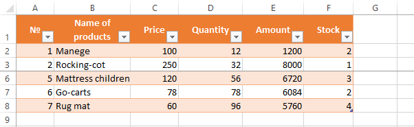
Usually an Excel table has one cap. Meanwhile, this document can have up to thousands of rows. Working with multipage table blocks is inconvenient when column names are not visible. Scrolling the page to its beginning to return to the correct cell is absolutely irrational. To make the cap visible when scrolling, fix the top row of the Excel table, following these actions:
- Create the needed table and fill it with the data.
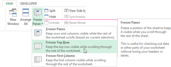
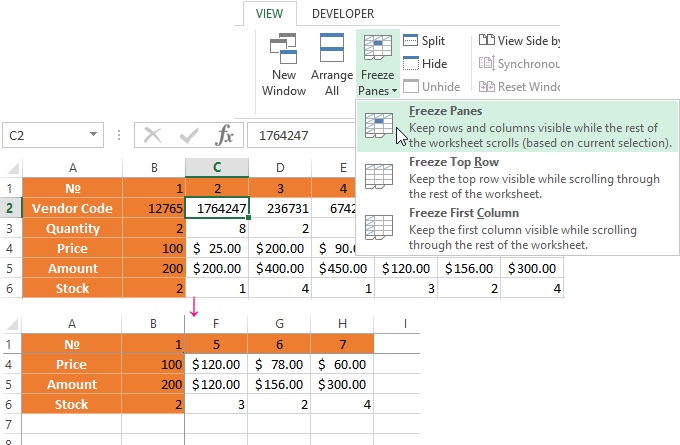
- Make any of the cells active. Go to the “VIEW” tab using the tool “Freeze Panes”.
- In the menu select the “Freeze Top Row” functions.
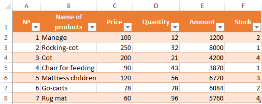
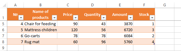
You will get a delimiting line under the top line. Now when you scroll vertically the table cap will be always visible.
Locking several rows in Excel while scrolling
Let us suppose, a user needs to fix not only the cap. For instance, another row or even a couple of rows must be fixed when scrolling the document. Doing it is possible and easy, when you follow these steps:
- Select any cell under the line, which we will fix. This action will help Excel to “understand”, which area should be fixed;
- Now select the “Freeze Panes” tool.
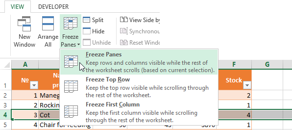
When you perform horizontal and vertical scrolling, the cap and the top row of the table remain fixed. Thus, you can fix two, three, four and more rows.
Note: This method works for 2007 and 2010 Excel versions. In earlier versions the “Lock areas” tool is located in the “Window” menu on the main page. There you must always (!) activate the cell under the freeze row.
Freezing columns in Excel
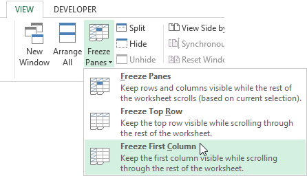
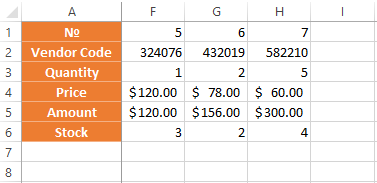
For instance, the information in the table has a horizontal direction. It is not concentrated in columns, but located in rows. For his comfort, the user must freeze the first column, containing the lines’ names in horizontal scrolling.
- Select any cell of the chosen table so that Excel understands with what data it will work. Pin the first column in the menu you will see..
- Now, when the document is scrolled to the right horizontally, the needed column will be fixed.
To freeze several columns, select the cell at the page bottom (to the right from the fixed column). Pick the “Freeze Panes” button.
How to freeze the row and column in Excel
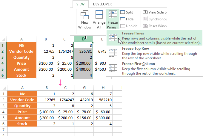
You have a task – to freeze the selected area, which contains two columns and two rows.
Make a cell at the intersection of the fixed rows and columns active. However, the cell must be not placed in the fixed area. It should have the position right under the required lines (to the right of the required columns). Pick the first option in Excel Locking Areas. The photo shows that when scrolling, the selected areas remain at the same place.
Removing a fixed area in Excel
After fixing a row or a column of the table the button deleting all pivot tables becomes available.
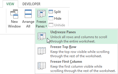
After clicking – «Unfreeze Panes», all the locked areas of the worksheet become unlocked.
Содержание
- How to fix a row and column in Excel when scrolling
- Locking a row in Excel while scrolling
- Locking several rows in Excel while scrolling
- Freezing columns in Excel
- How to freeze the row and column in Excel
- Removing a fixed area in Excel
- Freeze panes to lock rows and columns
- Freeze rows or columns
- Unfreeze rows or columns
- Need more help?
- Unhide the first column or row in a worksheet
- How to swap columns by dragging and other ways to move columns in Excel
- How to drag columns in Excel
- Swap Excel columns by cutting and pasting
- How to move one column in Excel
- How to move several columns in Excel
- Swap multiple columns by copying, pasting and deleting
- Change the columns order in Excel using VBA
- Re-arrange columns with Column Manager
How to fix a row and column in Excel when scrolling
The Microsoft Excel program is designed not only to enter data into the table conveniently and edit it as you need it, but also to view large blocks of information. Most people using PCs work with it constantly.
The columns and rows names can be significantly removed from the cells with which the user is working at this time. Scrolling the page to see the name of the document is not comfortable for any user. Therefore, the Tabular Processor has possibilities to fix certain areas.
Usually an Excel table has one cap. Meanwhile, this document can have up to thousands of rows. Working with multipage table blocks is inconvenient when column names are not visible. Scrolling the page to its beginning to return to the correct cell is absolutely irrational. To make the cap visible when scrolling, fix the top row of the Excel table, following these actions:
- Create the needed table and fill it with the data.

- Make any of the cells active. Go to the “VIEW” tab using the tool “Freeze Panes”.
- In the menu select the “Freeze Top Row” functions.
You will get a delimiting line under the top line. Now when you scroll vertically the table cap will be always visible.
Let us suppose, a user needs to fix not only the cap. For instance, another row or even a couple of rows must be fixed when scrolling the document. Doing it is possible and easy, when you follow these steps:
- Select any cell under the line, which we will fix. This action will help Excel to “understand”, which area should be fixed;
- Now select the “Freeze Panes” tool.
When you perform horizontal and vertical scrolling, the cap and the top row of the table remain fixed. Thus, you can fix two, three, four and more rows.
Note: This method works for 2007 and 2010 Excel versions. In earlier versions the “Lock areas” tool is located in the “Window” menu on the main page. There you must always (!) activate the cell under the freeze row.
Freezing columns in Excel
For instance, the information in the table has a horizontal direction. It is not concentrated in columns, but located in rows. For his comfort, the user must freeze the first column, containing the lines’ names in horizontal scrolling.
- Select any cell of the chosen table so that Excel understands with what data it will work. Pin the first column in the menu you will see..
- Now, when the document is scrolled to the right horizontally, the needed column will be fixed.
To freeze several columns, select the cell at the page bottom (to the right from the fixed column). Pick the “Freeze Panes” button.
How to freeze the row and column in Excel
You have a task – to freeze the selected area, which contains two columns and two rows.
Make a cell at the intersection of the fixed rows and columns active. However, the cell must be not placed in the fixed area. It should have the position right under the required lines (to the right of the required columns). Pick the first option in Excel Locking Areas. The photo shows that when scrolling, the selected areas remain at the same place.
Removing a fixed area in Excel
After fixing a row or a column of the table the button deleting all pivot tables becomes available.
After clicking – «Unfreeze Panes», all the locked areas of the worksheet become unlocked.
Источник
Freeze panes to lock rows and columns
To keep an area of a worksheet visible while you scroll to another area of the worksheet, go to the View tab, where you can Freeze Panes to lock specific rows and columns in place, or you can Split panes to create separate windows of the same worksheet.

Freeze rows or columns
Freeze the first column
Select View > Freeze Panes > Freeze First Column.
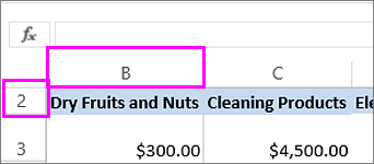
The faint line that appears between Column A and B shows that the first column is frozen.
Freeze the first two columns
Select the third column.
Select View > Freeze Panes > Freeze Panes.
Freeze columns and rows
Select the cell below the rows and to the right of the columns you want to keep visible when you scroll.
Select View > Freeze Panes > Freeze Panes.
Unfreeze rows or columns
On the View tab > Window > Unfreeze Panes.

Note: If you don’t see the View tab, it’s likely that you are using Excel Starter. Not all features are supported in Excel Starter.
Need more help?
You can always ask an expert in the Excel Tech Community or get support in the Answers community.
Источник
Unhide the first column or row in a worksheet
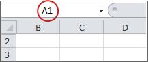
If the first row (row 1) or column (column A) is not displayed in the worksheet, it is a little tricky to unhide it because there is no easy way to select that row or column. You can select the entire worksheet, and then unhide rows or columns ( Home tab, Cells group, Format button, Hide & Unhide command), but that displays all hidden rows and columns in your worksheet, which you may not want to do. Instead, you can use the Name box or the Go To command to select the first row and column.
To select the first hidden row or column on the worksheet, do one of the following:
In the Name Box next to the formula bar, type A1, and then press ENTER.
On the Home tab, in the Editing group, click Find & Select, and then click Go To. In the Reference box, type A1, and then click OK.
On the Home tab, in the Cells group, click Format.
Do one of the following:
Under Visibility, click Hide & Unhide, and then click Unhide Rows or Unhide Columns.
Under Cell Size, click Row Height or Column Width, and then in the Row Height or Column Width box, type the value that you want to use for the row height or column width.
Tip: The default height for rows is 15, and the default width for columns is 8.43.
If you don’t see the first column (column A) or row (row 1) in your worksheet, it might be hidden. Here’s how to unhide it. In this picture column A and row 1 are hidden.
To unhide column A, right-click the column B header or label and pick Unhide Columns.
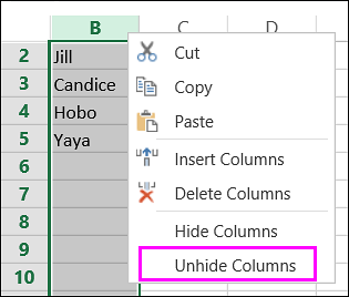
To unhide row 1, right-click the row 2 header or label and pick Unhide Rows.
Tip: If you don’t see Unhide Columns or Unhide Rows, make sure you’re right-clicking inside the column or row label.
Источник
How to swap columns by dragging and other ways to move columns in Excel
 by Svetlana Cheusheva, updated on February 7, 2023
In this article, you will learn a few methods to swap columns in Excel. You will see how to drag columns with a mouse and how to move a few non-contiguous columns at a time. The latter is often considered unfeasible, but in fact there’s a tool that allows moving non-adjacent columns in Excel 2016, 2013 and 2010 in a click.
If you extensively use Excel tables in your daily work, you know that whatever logical and well thought-out a table’s structure is, you have to reorder the columns every now and then. For example, you might need to swap a couple of columns to view their data side-by-side. Of course, you can try to hide the neighboring columns for a while, however this is not always the best approach because you may need to see data in those columns as well.
Surprisingly, Microsoft Excel does not provide a straightforward way to perform this common operation. If you try to simply drag a column name, which appears to be the most obvious way to move columns, you might be confused to find that it does not work.
All in all, there are four possible ways to switch columns in Excel, namely:
How to drag columns in Excel
As already mentioned, dragging columns in Excel is a bit more complex procedure than one could expect. In fact, it’s one of those cases that can be classified as «easier said than done». But maybe it’s just my lack of sleight of hand ability 🙂 Nevertheless, with some practice, I was able to get it to work, so you will definitely manage it too.
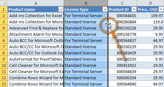
Suppose, you have a worksheet with information about your company’s products and you want to quickly swap a couple of columns there. I will use the AbleBits price list for this example. What I want is to switch the «License type» and «Product ID» columns so that a product ID comes right after the product name. 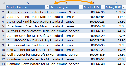
- Select the column you want to move.
- Put the mouse pointer to the edge of the selection until it changes from a regular cross to a 4-sided arrow cursor. You’d better not do this anywhere around the column heading because the cursor can have too many different shapes in that area. But it works just fine on the right or left edge of the selected column, as shown in the screenshot.
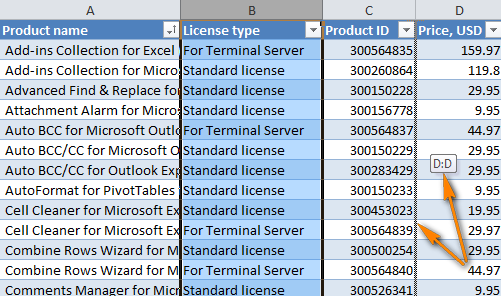
- Press and hold the Shift key, and then drag the column to a new location. You will see a faint «I» bar along the entire length of the column and a box indicating where the new column will be moved.
- That’s it! Release the mouse button, then leave the Shift key and find the column moved to a new position.
You can use the same technique to drag several columns in your Excel table. To select several columns, click the heading of the first column you need to move, press and hold Shift , and then click the heading of the last column. Then follow steps 2 — 4 above to move the columns, as shown in the screenshot. 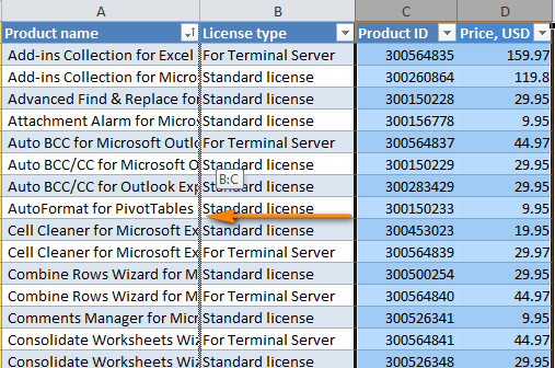
Note. It is not possible to drag non-adjacent columns and rows in Excel.
The drag and drop method works in Microsoft Excel 2016, 2013, 2010 and 2007 and can be used for moving rows as well. It might require some practice, but once mastered it could be a real time saver. Though, I guess the Microsoft Excel team will hardly ever win an award for the most user friendly interface on this feature 🙂
Swap Excel columns by cutting and pasting
If manipulating the mouse pointer is not your technique of choice, then you can change the columns order by cutting and pasting them. Please keep in mind that there’re a few tricks here depending on whether you want to move a single column or several columns at a time:
How to move one column in Excel
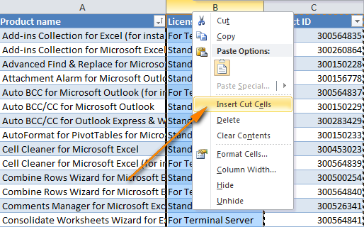
- Select the entire column by clicking on the column header.
- Cut the selected column by pressing Ctlr + X , or right click the column and choose Cut from the context menu. You can actually skip step 1 and simply right click the column’s heading to choose Cut.
- Select the column before which you want to insert the cut column, right click it and choose Insert Cut Cells from the pop-up menu.
If you are more comfortable with Excel shortcuts and keyboard, then you may like the following way to move columns in Excel:
- Select any cell in the column and press Ctrl + Space to select the whole column.
- Hit Ctrl + X to cut the column.
- Select the column before which you what to paste the cut column.
- Press Ctrl together with the Plus sign (+) on the numeric keypad to insert the column.
How to move several columns in Excel
The cut / paste method that works just fine for a single column does not allow switching several columns at a time. If you try to do this, you will end up with the following error: The command you chose cannot be performed with multiple selections.
To reorder a few columns in your worksheet, choose one of the following options:
- Drag several columns using the mouse (in my opinion, this is the fastest way).
- Cut and paste each column individually (probably not the best approach if you have to move a lot of columns).
- Copy, paste and delete (allows moving several adjacent columns at a time).
Swap multiple columns by copying, pasting and deleting
If dragging columns with a mouse does not work for you for some reason, then you can try to re-arrange several columns in your Excel table is this way:
- Select the columns you want to switch (click the first column’s heading, press Shift and then click the last column heading).
An alternative way is to select only the headings of the columns to be moved and then press Ctrl + Space . This will select only cells with data rather than entire columns, as shown in the screenshot below. 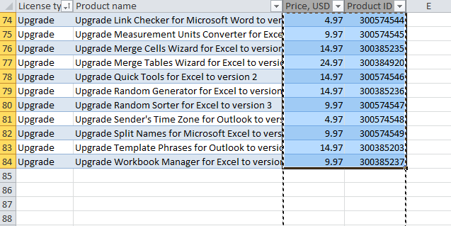
Note. If you are re-arranging columns in a range, either way will do. If you are to swap a few columns in an Excel table, then select the columns using the second way (cells with data only), otherwise you may get the error «The operation is not allowed. The operation is attempting to shift cells in a table of your worksheet».
Of course, this is a bit longer process compared to dragging columns, but it may work for those who prefer shortcuts to fiddling with the mouse. Regrettably, it does not work for non-contingent columns either.
Change the columns order in Excel using VBA
If you have some knowledge of VBA, you can try to write a macro that would automate moving columns in your Excel sheets. This is in theory. In practice, most likely you would end up spending more time on specifying which exactly columns to swap and defining their new placements than dragging the columns manually. Besides, there is no guarantee that the macro will always work as expected and each time you would need to verify the result anyways. All in all, a VBA macro does not seem to be well-suited for this task.
Re-arrange columns with Column Manager
If you are looking for a fast and reliable tool to switch columns in your Excel sheets, the Column Manager included with our Ultimate Suite is certainly worth your attention. It lets you change the order of columns on the fly, without manual copying / pasting or learning a handful of shortcuts.
With the Ultimate Suite installed in your Excel, click the Colum Manager button on the Ablebits Data tab, in the Manage group: 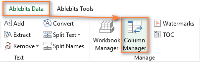
The Column Manager’s pane will appear in the right side of the Excel window and displays a list of columns that are present in your active worksheet.
To move one or more columns, select them on the pane and click the Up or Down arrow on the toolbar. The former moves the selected columns to the left in your sheet, the latter to the right: 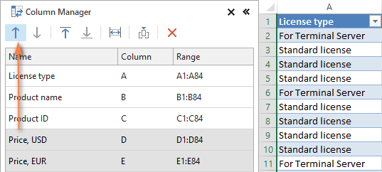
Or, drag-and-drop the columns on the pane with your mouse. Both methods work for adjacent and non-adjacent columns: 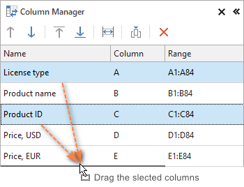
All the manipulations that you do on the Colum Manager pane are simultaneously performed on your worksheet, which lets you visually see all the changes and have full control over the process.
Another truly wonderful feature is the ability to move a single column or multiple columns to the beginning (far left) or to the end (far right) of the table in a click: 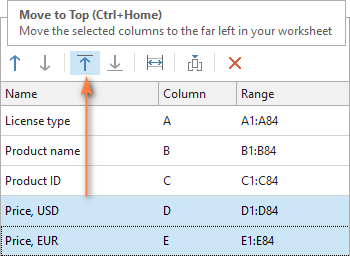
And finally, a couple of nice bonuses:
 — Click this icon to auto fit the width of the selected columns.
 — Click this icon to insert a new column.
I have to admit that I really love this little smart add-in. Together with the other 70+ tools included in the Ultimate Suite, it makes common operations in Excel not only faster and easier, but actually enjoyable. Of course, you should not take my words for granted because I’ve got used to them and therefore am sort of biased 🙂
So, go ahead and download a trial version to see for yourself.
Источник
You want to keep an
area of a large Excel worksheet visible while you scroll to another area of the
worksheet, then you should to fix/freeze row(s) or/and column(s).
Fix/Freeze the first/top row:
1.
From the View tab, Window
Group, click the Freeze Panes drop down arrow.
2.
Select Freeze Top Row
(View > Freeze
Panes > Freeze Top Row)

Excel inserts a thin
line between row 1 and row 2 to show you where the frozen pane begins

Fix/Freeze rows:
To fix/freeze several
rows:
Select the row immediately below the last row you want to
freeze.
1.
From the View tab, Window
Group, click the Freeze Panes drop down arrow.
2.
Select Freeze Panes
(View > Freeze
Panes > Freeze Panes)
Excel inserts a thin
line to show you where the frozen pane begins
Unfix / unfreeze row(s):
To unfreeze and restore
the workbook to its normal view:
Select View
tab, Window Group, click Freeze Panes and select Unfreeze
Panes .

Last Updated: February 8, 2022 | Author: Edwin Heist
How do I freeze specific rows and columns in Excel?
Freeze columns and rows
- Select the cell below the rows and to the right of the columns you want to keep visible when you scroll.
- Select View > Freeze Panes > Freeze Panes.
What is the shortcut to fix a row in Excel?
Here are the shortcuts for freezing rows/columns:
- To freeze the top row: ALT + W + F + R. Note that the top row gets fixed.
- To freeze the first column: ALT + W + F + C. Note that the left-most column gets fixed.
How do I keep a row from moving in Excel?
How to freeze a set of rows in Excel
- Select the row below the set of rows you want to freeze.
- In the menu, click “View.”
- In the ribbon, click “Freeze Panes” and then click “Freeze Panes.”
How do I unfreeze a row in Excel?
To unfreeze panes:
To unfreeze rows or columns, click the Freeze Panes command, then select Unfreeze Panes from the drop-down menu.
How do I fix a specific column in Excel?
Select the column that’s immediately to the right of the last column you want frozen. Select the View tab, Windows Group, click the Freeze Panes drop down and select Freeze Panes. Excel inserts a thin line to show you where the frozen pane begins.
How do I lock a row in sheets?
Freeze or unfreeze rows or columns
- On your computer, open a spreadsheet in Google Sheets.
- Select a row or column you want to freeze or unfreeze.
- At the top, click View. Freeze.
- Select how many rows or columns to freeze.
How do I freeze a selected row?
To freeze rows:
- Select the row below the row(s) you want to freeze. In our example, we want to freeze rows 1 and 2, so we’ll select row 3. …
- Click the View tab on the Ribbon.
- Select the Freeze Panes command, then choose Freeze Panes from the drop-down menu. …
- The rows will be frozen in place, as indicated by the gray line.
How do you keep a cell fixed in Excel?
Keep formula cell reference constant with the F4 key
1. Select the cell with the formula you want to make it constant. 2. In the Formula Bar, put the cursor in the cell which you want to make it constant, then press the F4 key.
What is a row vs column?
What is the Difference between Rows and Columns?
| Rows | Columns |
|---|---|
| A row can be defined as an order in which objects are placed alongside or horizontally | A column can be defined as a vertical division of objects on the basis of category |
| The arrangement runs from left to right | The arrangement runs from top to bottom |
•
Jul 2, 2020
How do you link rows to columns in Excel?
How to use the macro to convert row to column
- Open the target worksheet, press Alt + F8, select the TransposeColumnsRows macro, and click Run.
- Select the range that you want to transpose and click OK:
- Select the upper left cell of the destination range and click OK:
How do I unfreeze a row in Google Sheets?
Freeze or unfreeze rows or columns
- On your Android phone or tablet, open a spreadsheet in the Google Sheets app.
- Touch and hold a row or column.
- In the menu that appears, tap Freeze or Unfreeze.
Are rows up and down?
A row is a series of data put out horizontally in a table or spreadsheet while a column is a vertical series of cells in a chart, table, or spreadsheet. Rows go across left to right. On the other hand, Columns are arranged from up to down.
What is a row in Excel?
In Microsoft Excel, a row runs horizontally in the grid layout of a worksheet. Horizontal rows are numbered with numeric values such as 1, 2, 3. … Each row in the worksheet has its own row number which is used as part of a cell reference such as A1, A2, or M16.
How do you add a row in Excel?
To insert a single row: Right-click the whole row above which you want to insert the new row, and then select Insert Rows. To insert multiple rows: Select the same number of rows above which you want to add new ones. Right-click the selection, and then select Insert Rows.
What ways are rows?
Rows are arranged horizontally, from left to right, while columns are arranged vertically, from top to bottom.
How can I delete a row in Excel?
Keyboard shortcut to delete a row in Excel
- Shift+Spacebar to select the row.
- Ctrl+-(minus sign) to delete the row.
Which way does rows go in Excel?
MS Excel is in tabular format consisting of rows and columns.
- Row runs horizontally while Column runs vertically.
- Each row is identified by row number, which runs vertically at the left side of the sheet.
- Each column is identified by column header, which runs horizontally at the top of the sheet.
What do rows start with?
The column always goes first followed by the row, without a space. This naming convention is true not only in word of mouth and writing but when making formulas in a spreadsheet.
How are rows labeled in Excel?
By default, Excel uses the A1 reference style, which refers to columns as letters (A through IV, for a total of 256 columns), and refers to rows as numbers (1 through 65,536). These letters and numbers are called row and column headings. To refer to a cell, type the column letter followed by the row number.
Skip to content
При работе с большими наборами данных в Excel вам может потребоваться заблокировать определенные строки или столбцы, чтобы вы могли видеть их содержимое при прокрутке в другую область рабочего листа. Ниже вы найдете подробные инструкции о том, как закрепить одну или несколько строк, зафиксировать один или несколько столбцов или «заморозить» и то, и другое одновременно, а также как снять блокировку. В Excel есть специальные инструменты, чтобы зафиксировать шапку таблицы, первые столбцы или же и то, и другое сразу.
Возможность закрепить строку — очень важный лайфхак в Экселе. Научившись этому простому приему, вы сможете просматривать любую область таблицы, не теряя из поля зрения строку с именами столбцов или так называемую «шапку» таблицы.
Это можно легко сделать с помощью меню Закрепить области и нескольких других функций.
Итак, как закрепить строку в Excel? Разберём самое важное:
- Как зафиксировать вернюю строку при прокрутке
- Как зафиксировать сразу несколько строк.
- Закрепляем крайний левый столбец.
- Как закрепить по вертикали и горизонтали одновременно?
- Что если нужно отменить?
- Почему не работает?
- Нетрадиционные спрсобы фиксации строк и столбцов
- Если нужно зафиксировать заголовок таблицы при печати
- Будьте аккуратны — несколько советов и предупреждений
«Замораживание» на экране части информации — это всего лишь несколько щелчков мышью. Вы просто нажимаете вкладку «Вид» > ![]() и выбираете один из параметров в зависимости от того, что вы хотите заблокировать (как на скриншоте ниже).
и выбираете один из параметров в зависимости от того, что вы хотите заблокировать (как на скриншоте ниже).
А теперь объясним подробнее.
Как закрепить верхнюю строку в Excel.
Если ваша таблица содержит большое количество строк, то при прокрутке вниз шапка с названиями колонок скроется из виду. И вам будет достаточно сложно ориентироваться в изобилии цифр. Ведь довольно сложно запомнить, что записано в каждом из столбцов. Или придется постоянно прокручивать таблицу вверх-вниз. Поэтому эту проблему нужно обязательно решить, закрепив одну или несколько верхних строк таблицы.
Рассмотрим, как зафиксировать строку в Excel при прокрутке таблицы вниз. Перейдите на вкладку «Вид» и действуйте так, как показано на рисунке.
Это действие заблокирует самую первую строку в вашем рабочем листе Excel, чтобы она оставалась на виду при навигации по данным.
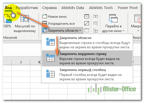
Вы можете визуально определить, что шапка таблицы «заморожена», видя серую линию под ней:

Как «заморозить» несколько строк.
Но очень часто бывает, что шапка таблицы расположена в нескольких верхних строках. Если вы хотите заблокировать несколько строчек (начиная с первой), то выполните следующие действия:
- Выберите строку (или просто первую позицию в ней), информацию выше которой вы хотите видеть постоянно. Например, если заголовки столбцов занимают первые две строки, то установите курсор в первую ячейку третьей строки.
- На вкладке «Вид» нажмите

Например, чтобы заблокировать две верхние строки на листе, мы выбираем ячейку A3 и выбираем первый пункт в меню:

Как видно на скриншоте, если мы хотим зафиксировать первые две строчки, устанавливаем курсор на третью. В результате вы сможете прокручивать содержимое листа, а на экране всегда будет оставаться шапка таблицы.
Предупреждения:
- Учтите, что при закреплении области таблицы будут зафиксированы все строки и столбцы, которые находятся выше и левее указанной ячейки. Поэтому, если вы хотите закрепить только строки, то установите курсор в ячейку первого столбца перед использованием инструмента.
- Microsoft Excel при прокрутке таблицы позволяет замораживать только содержимое верхней части рабочего листа. Невозможно заблокировать что-либо в середине.
- Убедитесь, что все фиксируемые данные видны в момент «замораживания». Если какие-то данные не видны, то они будут скрыты.
- Если вы вставите строку перед той, что была закреплена (в нашем случае, между первой и второй), то она тоже будет зафиксирована.
Как зафиксировать столбец в Excel
Теперь рассмотрим, как закрепить столбец в Excel при прокрутке вправо. Эта операция выполняется аналогично рассмотренным выше действиям со строками.
Как заблокировать первый столбец.
Чтобы закрепить столбец при прокрутке вправо, выберите в выпадающем меню — «Закрепить первый столбец».
Это сделает первую слева колонку постоянно видимой во время горизонтальной прокрутки вправо.
Как «заморозить» несколько столбцов.
Чтобы зафиксировать более одного столбца, это то, что вам нужно сделать:
- Выберите столбец (или первую позицию в нем) справа от последнего столбца, который вы хотите заблокировать.
- Перейдите на вкладку «Вид» и нажмите
Например, чтобы заморозить первые два столбца, выделите всю колонку C или просто поставьте курсор в ячейку C1 и нажмите как на скриншоте:

Это позволит вам постоянно видеть первые 2 позиции с левой стороны при перемещении по рабочему листу.
Предупреждения:
- Вы можете закрепить столбец только слева, на краю вашей таблицы. Столбцы в середине таблицы не могут быть зафиксированы.
- Все столбцы, которые нужно заблокировать, должны быть видны. Все, которые не видны, будут скрыты после фиксации.
- Если вы вставите колонку перед той, что была закреплена, новая колонка будет также закрепленной. В нашем примере, если вы вставите столбец между A и B, то Excel при прокрутке зафиксирует уже 3 первых столбца.
Как закрепить строку и столбец одновременно.
Помимо блокировки по отдельности, Microsoft Excel позволяет замораживать одновременно ячейки по вертикали и горизонтали. Вот как делается закрепление областей :
- Выберите клетку ниже и справа от той области, которую вы хотите заблокировать. К примеру, если мы хотим постоянно видеть на экране шапку таблицы, состоящую из двух строчек, а также первые две колонки слева, то ставим курсор в C3.
- На вкладке «Вид» выберите .

Да, это так просто 
Таким же образом вы можете заморозить столько по вертикали и горизонтали, сколько захотите. Но при условии, что вы начинаете с верхнего ряда и самой левой колонки.
Например, чтобы заблокировать верхнюю строку и первые 2 столбика, вы выбираете C2; чтобы заморозить первые две строчки и первые две колонки, выберите C3 и т. д.
Обратите внимание, что, чтобы закрепить строку и столбец, действуют те же правила, о которых мы говорили выше. Зафиксировано будет только то, что видно на экране. Все, что находится выше и правее и не попадает на экран на момент совершения операции, будет просто скрыто.
Как разблокировать строки и столбцы?
Если вы «заморозили» часть таблицы, то нажатием горячих клавиш Ctrl+Z (отмена действия) нельзя ничего исправить. Снять закрепление областей можно только через меню.
Чтобы разблокировать «зафиксированные» данные, перейдите на вкладку «Вид» и нажмите «Снять закрепление …». Эта кнопка появляется в меню, только если вы закрепили какие-то строки либо столбцы.

При этом уже не важно, где расположен курсор и в каком месте листа вы находитесь.
Почему не работает?
Если кнопка ![]() отключена (выделена серым цветом) то, скорее всего, это происходит по следующим причинам:
отключена (выделена серым цветом) то, скорее всего, это происходит по следующим причинам:
- Вы находитесь в режиме редактирования. Например, происходит ввод формулы или редактирование данных. Чтобы выйти из режима редактирования, нажмите Enter или Esc.
- Ваш рабочий лист защищен. Пожалуйста, сначала снимите защиту рабочей книги, а затем действуйте, как описано выше в этой статье.
Другие способы закрепления столбцов и строк.
Еще один способ несколько нестандартный способ — это разделить экран на несколько частей. Особенность этого приёма заключается в следующем:
Разделение панелей делит ваш экран на две или же четыре области, которые можно просматривать независимо друг от друга. При прокрутке внутри одной из них ячейки в другой остаются на прежнем месте.
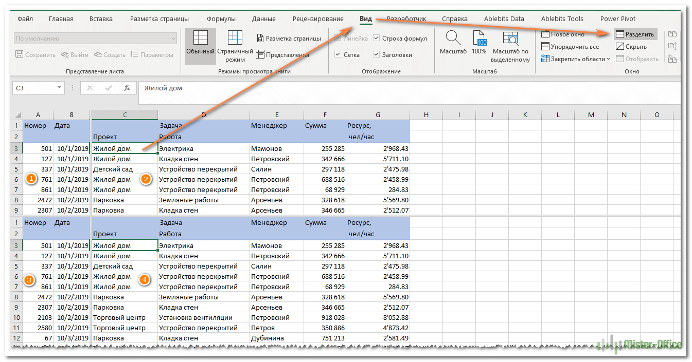
Чтобы разделить окно на части, выберите позицию снизу или справа от того места, в котором вы хотите это сделать, и нажмите соответствующую кнопку. Чтобы отменить операцию, снова нажмите её же.
Еще один способ — использование «умной» таблицы для блокировки её заголовка.
Если вы хотите, чтобы заголовок всегда оставался фиксированным вверху при прокрутке вниз, преобразуйте диапазон в таблицу Excel:
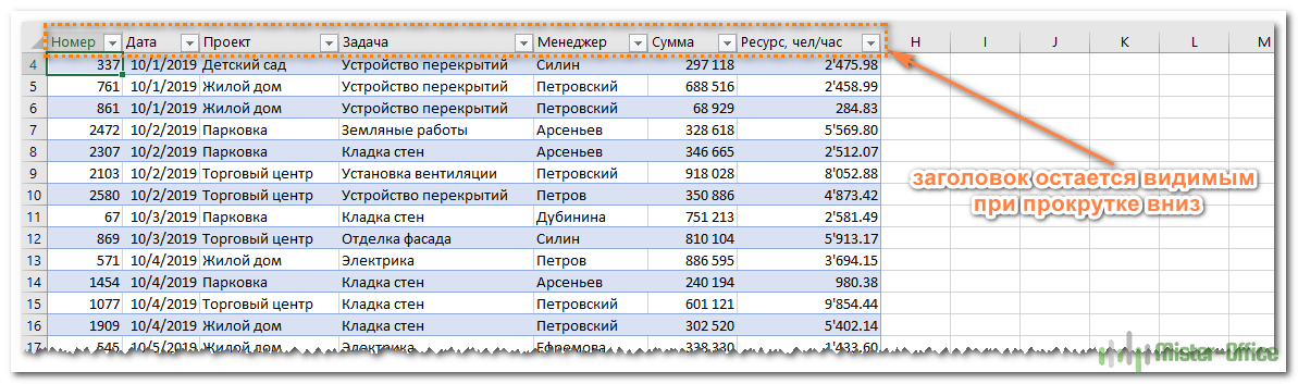
Самый быстрый способ создать таблицу в Excel — нажать Ctl + T.
Однако при этом учитывайте, что если шапка состоит более чем из 1 строчки, то зафиксируется только первая из них. В результате может получиться не очень красиво.
Печать заголовка таблицы на каждой странице
Если вы хотите повторить одну или несколько верхних строк листа Excel на каждой напечатанной странице, переключитесь на вкладку «Разметка страницы» и нажмите кнопку «Печатать заголовки». Далееперейдите на вкладку «Лист» и выберите сквозные строки.
Несколько советов и предупреждений.
Как вы только что видели, фиксация областей в Excel — одна из самых простых задач. Однако, как это часто бывает с Microsoft, внутри скрывается гораздо больше.
Предостережение: предотвращение полного исчезновения строк и столбцов при закреплении областей рабочей книги.
Когда вы блокируете несколько строк или столбцов в электронной таблице, вы можете непреднамеренно скрыть некоторые из них, и в результате потом вы уже не увидите их. Чтобы избежать этого, убедитесь, что всё, что вы хотите зафиксировать, находится в поле зрения в момент осуществления операции.
Например, вы хотите заморозить первые две строчки, но первая в настоящее время не видна, как показано на скриншоте ниже. В результате первая из них не будет отображаться позже, и вы не сможете переместиться на нее. Тем не менее, вы все равно сможете установить курсор в ячейку в скрытой замороженной позиции с помощью клавиш управления курсором (которые со стрелками) и при необходимости даже изменить её.

Excel может зафиксировать области несколько иначе, чем вы ожидали.
Вы мне не верите? Тогда попробуйте выбрать ячейку A3, когда первые две не видны (просто находятся чуть выше видимой части таблицы), и щелкните ![]() . Что вы ожидаете? Что строки 1 — 2 будут заморожены? Нет! Microsoft Excel думает иначе, и на снимке экрана ниже показан один из многих возможных результатов:
. Что вы ожидаете? Что строки 1 — 2 будут заморожены? Нет! Microsoft Excel думает иначе, и на снимке экрана ниже показан один из многих возможных результатов:
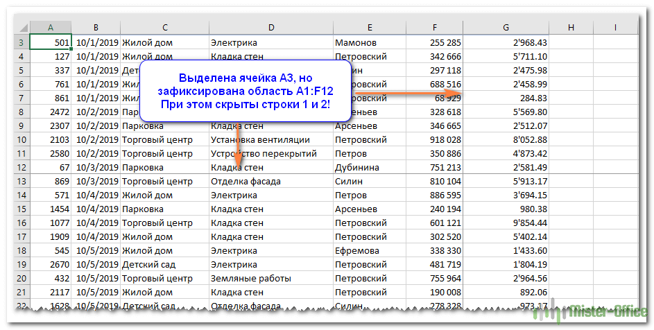
Неподвижной стали ¾ экрана. Вряд ли с такой логикой программы можно согласиться.
Поэтому, пожалуйста, помните, что данные, которые вы собираетесь зафиксировать, всегда должны быть полностью видны.
Совет: Как замаскировать линию, отделяющую закрепленную область.
Если вам не нравится тёмная линия, которую Microsoft Excel рисует внизу и справа от зафиксированной области, вы можете попытаться замаскировать ее с помощью шаблонов оформления и небольшого творческого подхода:)

Выберите приятный для вас вариант оформления нижней границы ячеек, и линия не будет раздражать вас.
Вот как вы можете заблокировать строку в Excel, зафиксировать столбец или одновременно сделать и то, и другое.
И это все на сегодня. Спасибо, что прочитали!