Fix formula cells in excel

I want to cover something today that I use all of the time but seems to be understood in varying degrees by clients I work with.

I am talking about use of the dollar sign ($) in an Excel formula.

Relative cell references
When you copy and paste an Excel formula from one cell to another, the cell references change, relative to the new position:

EXAMPLE:

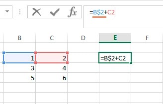
If we have the very simple formula «=A1» in cell B1 it will change as follows when copied and pasted:

Pasted to B2, it becomes «=A2»

Pasted to C2, it becomes «=B2»

Pasted to A2, it returns an error!

In each case it is changing the reference to refer to the cell one to the left on the same row as the cell that the formula is in, i.e. the same relative position that A1 was to the original formula.

The reason an error is returned when it is pasted into column A, is because there are no columns to the left of column A.

This behaviour is very useful and is what allows a sum to be copied across or down the page and automatically refer to the new column or row that it finds itself in.

But in some situations, you want some or all of the references to remain fixed when they are copied elsewhere.

The dollar sign ($)
This is where the dollar sign is used.

EXAMPLE:

Take an example where you have a column of Sales values in Pounds Sterling in column A and a formula to convert these into US Dollars in column B. You could enter the actual exchange rate into the formula but it would be more sensible to refer to a cell where the exchange rate is held, so that it can be updated whenever it is needed.

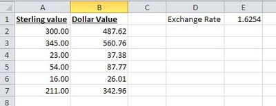
The simple formula for cell B2, would be «=A2*E1», however if you copy this down, then the formula in cell B3, would read «=A3*E2» as both references would move down a row as described above.

This is where the dollar sign ($) is used. The dollar sign allows you to fix either the row, the column or both on any cell reference, by preceding the column or row with the dollar sign. In our example if we replace the formula in cell B2 with «=A2*$E$1», then both the «E» and the «1» will remain fixed when the formula is copied. i.e. in cell B3, the formula will read «=A3*$E$1», still referring to the cell with the exchange rate in it.

In this example we have fixed both the row and the column, but in other situations, you may just want to fix one or the other, for example:

Above we have a spreadsheet calculating the times tables where we want to every cell in the white area to be the product of its row and column heading. This is easy using the dollar symbol. In cell B2, the formula without dollars would be «=A2*B1», but for this formula to work when copied to each column, we need it to always look at column A for the first reference and to work for each row, we need to always look at row 1 for the second. Using the dollar sign to do this, it becomes «=$A2*B$1». This can then be copied to every cell in the white area.

Quick Tip
You can speed up entering the dollar signs by using the function key F4 when editing the formula, if the cursor is on a cell reference in the formula, repeatedly hitting the F4 key, toggles between no dollar signs, both dollar signs, just the row and just the column.

If you enjoyed this post, go to the top of the blog, where you can subscribe for regular updates and get your free report «The 5 Excel features that you NEED to know».

Источник

The advantages of absolute references are difficult to underestimate. They often have to be used in the process of working with the program. Relative references to cells in Excel are more popular than absolute ones, but they also have their pros and cons.

In Excel, there are several types of links: absolute, relative and mixed. This also includes «names» for whole ranges of cells. Consider their possibilities and differences in practical application in formulas.

Absolute and relative links in Excel

Absolute references allow us to fix a row or column (or row and column at a time) to which the formula should refer. Relative references in Excel change automatically when you copy a formula along a range of cells, both vertically and horizontally. A simple example of relative cell addresses. Let us calculate the volume of the sphere in Excel:

Fill the range of cells A2: A5 with different radii.
In cell B2, enter the formula for calculating the volume of the sphere, which will refer to the value of A2. The formula will look like this: =(4/3)*3.14*A2^3
Copy the formula from B2 along column A2: A5.

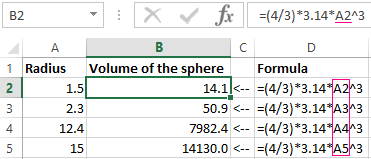
As you can see, the relative addresses help to change the address in each formula automatically.

It is also worth to point the regularity of changes in references of formulas. Data in B3 refers to A3, B4 to A4, and so on. Everything depends on where the first introduced formula will refer, and its copies will change the references relative to its position in the range of cells on the sheet.

Now instead of numbers we use absolute references:

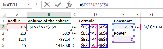
The result of the calculation is the same, but the formulas are more flexible to the changes. It is enough to change the value in one cell and the whole column is recalculated automatically. See the following example.

Use of absolute and relative links in Excel

Fill in the plate, as shown in the picture:

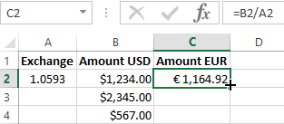
Description of the source table. In cell A2, there is an actual euro exchange rate against the dollar for today. In the range of cells B2: B4 are the amounts in dollars. In the range C2: C4 will be the amount in euros after the conversion of currencies. Tomorrow the course will change and the task of the plate will automatically recalculate the range of C2: C4 depending on the change in the value in cell A2 (that is, the euro rate).

To solve this problem, we need to enter a formula in C2: = B2 / A2 and copy it to all cells in the C2: C4 range. But here there is a problem. From the previous example, we know that when copying, relative references automatically change addresses relative to their position. Therefore, an error occurs:

error.

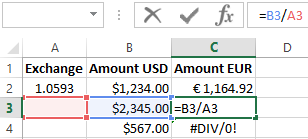
Concerning the first argument, this is quite acceptable. After all, the formula automatically refers to the new value in the column of the table cells (dollar amounts). But the second indicator we need to fix on the address A2. Accordingly, it is necessary to change the relative reference to the absolute in the formula.

How to make an absolute reference in Excel? It is very simple to put the $ (dollar) symbol before the line or column number or before the both of them. Below, consider all 3 options and determine their differences.

Our new formula should contain at once 2 types of links: absolute and relative.

In C2, enter another formula: = B2 / A $ 2. To change links in Excel, double click on the cell with the left mouse button or press the F2 key on the keyboard.
Copy it to the other cells in the C3:C4 range.

Done.

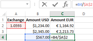
Description of the new formula. The dollar symbol ($) in the address of references fixes the address in the new copied formulas.

Absolute, relative and mixed references in Excel:

$ A $ 2 — address of the absolute reference with fixation on columns and rows, both vertically and horizontally.
$ A2 is a mixed link. When copying a column is fixed, and the row is changed.
A $ 2 is a mixed link. When copying a row is fixed, and the column is changed.

For comparison: A2 is a relative address, without fixation. During the copying of the formulas, the row (2) and the column (A) automatically change to the new addresses relative to the location of the copied formula, both vertically and horizontally.

Note. In this example, the formula can contain not only a mixed link, but the absolute result: = B2 / $ A $ 2. The result will be the same. But in practice, there are often cases when you cannot do a thing without mixed references.

Helpful advice. To avoid entering the dollar symbol ($) manually, after specifying the address, press F4 repeatedly to select the required type: absolute or mixed. It’s fast and convenient.

Источник

How to avoid broken formulas

Excel for Microsoft 365 Excel for Microsoft 365 for Mac Excel for the web Excel 2021 Excel 2021 for Mac Excel 2019 Excel 2019 for Mac Excel 2016 Excel 2016 for Mac Excel 2013 Excel for iPad Excel for Android tablets Excel 2010 Excel 2007 Excel Starter 2010 More…Less

If Excel can’t resolve a formula you’re trying to create, you may get an error message like this one:

Unfortunately, this means that Excel can’t understand what you’re trying to do, so you’ll need to update your formula or make sure you’re using the function correctly.

Tip: There are a few common functions where you might run into issues, check out COUNTIF, SUMIF, VLOOKUP, or IF to learn more. You can also see a list of functions here.

Return to the cell with the broken formula, which will be in edit mode, and Excel will highlight the spot where it’s having a problem. If you still don’t know what to do from there and want to start over, you can press ESC again, or select the Cancel button in the formula bar, which will take you out of edit mode.

If you want to move forward, then the following checklist provides troubleshooting steps to help you figure out what may have gone wrong. Select the headings to learn more.

Note: If you’re using Microsoft 365 for the web, you may not see the same errors, or the solutions may not apply.

Excel throws a variety of pound (#) errors such as #VALUE!, #REF!, #NUM, #N/A, #DIV/0!, #NAME?, and #NULL!, to indicate something in your formula isn’t working properly. For example, the #VALUE! error is caused by incorrect formatting or unsupported data types in arguments. Or, you’ll see the #REF! error if a formula refers to cells that have been deleted or replaced with other data. Troubleshooting guidance will differ for each error.

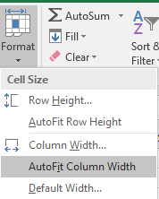
Note: #### is not a formula-related error. It just means that the column isn’t wide enough to display the cell contents. Simply drag the column to widen it, or go to Home > Format > AutoFit Column Width.

Refer to any of the following topics corresponding to the pound error you see:

Correct a #NUM! error
Correct a #VALUE! error
Correct a #N/A error
Correct a #DIV/0! error
Correct a #REF! error
Correct a #NAME? error
Correct a #NULL! error

Each time you open a spreadsheet that contains formulas referring to values in other spreadsheets, you’ll be prompted to update the references or leave them as-is.

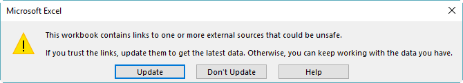
Excel displays the above dialog box to make sure that the formulas in the current spreadsheet always point to the most updated value in case the reference value has changed. You can choose to update the references, or skip if you don’t want to update. Even if you choose to not update the references, you can always manually update the links in the spreadsheet whenever you want.

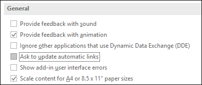
You can always disable the dialog box from appearing at start up. To do that, go to File > Options > Advanced > General, and clear the Ask to update automatic links box.

Important: If this is the first time you’re working with broken links in formulas, if you need a refresher on resolving broken links, or if you don’t know whether to update the references, see Control when external references (links) are updated.

If the formula doesn’t display the value, follow these steps:

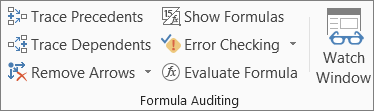
Make sure Excel is set to show formulas in your spreadsheet. To do this, select the Formulas tab, and in the Formula Auditing group, select Show Formulas.

Tip: You can also use the keyboard shortcut Ctrl + ` (the key above the Tab key). When you do this, your columns will automatically widen to display your formulas, but don’t worry, when you toggle back to the normal view, your columns will resize.
If the step above still doesn’t resolve the issue, it’s possible the cell is formatted as text. You can right-click on the cell and select Format Cells > General (or Ctrl + 1), then press F2 > Enter to change the format.
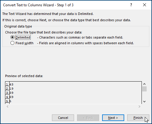
If you have a column with a large range of cells that are formatted as text, you can select the range, apply the number format of your choice, and go to Data > Text to Column > Finish. This will apply the format to all of the selected cells.

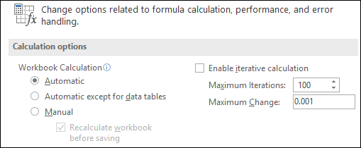
When a formula does not calculate, you’ll need to check if automatic calculation is enabled in Excel. Formulas won’t calculate if manual calculation is enabled. Follow these steps to check for Automatic calculation.

Select the File tab, select Options, and then select the Formulas category.
In the Calculation options section, under Workbook Calculation, make sure the Automatic option is selected.

For more information on calculations, see Change formula recalculation, iteration, or precision.

A circular reference occurs when a formula refers to the cell that it’s located in. The fix is to either move the formula to another cell, or change the formula syntax to one that avoids circular references. However, in some scenarios you may need circular references because they cause your functions to iterate—repeat until a specific numeric condition is met. In such cases, you’ll need to enable Remove or allow a circular reference.

For more information on circular references, see Remove or allow a circular reference.

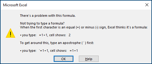
If your entry doesn’t start with an equal sign, it isn’t a formula, and won’t be calculated—a common mistake.

When you type something like SUM(A1:A10), Excel shows the text string SUM(A1:A10) instead of a formula result. Alternatively, if you type 11/2, Excel shows a date, such as 2-Nov or 11/02/2009, instead of dividing 11 by 2.

To avoid these unexpected results, always start the function with an equal sign. For example, type: =SUM(A1:A10) and =11/2.

When you use a function in a formula, each opening parenthesis needs a closing parenthesis for the function to work correctly. Make sure that all parentheses are part of a matching pair. For example, the formula =IF(B5<0),»Not valid»,B5*1.05) won’t work because there are two closing parentheses, but only one opening parenthesis. The correct formula would look like this: =IF(B5<0,»Not valid»,B5*1.05).

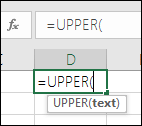
Excel functions have arguments—values you need to provide for the function to work. Only a few functions (such as PI or TODAY) take no arguments. Check the formula syntax that appears as you start typing in the function, to make sure the function has the required arguments.

For example, the UPPER function accepts only one string of text or cell reference as its argument: =UPPER(«hello») or =UPPER(C2)

Note: You’ll see the function’s arguments listed in a floating function reference toolbar beneath the formula as you’re typing it.

Also, some functions, such as SUM, require numerical arguments only, while other functions, such as REPLACE, require a text value for at least one of their arguments. If you use the wrong data type, functions might return unexpected results or show a #VALUE! error.

If you need to quickly look up the syntax of a particular function, see the list of Excel functions (by category).

Don’t enter numbers formatted with dollar signs ($) or decimal separators (,) in formulas because dollar signs indicate Absolute References and commas are argument separators. Instead of entering $1,000, enter 1000 in the formula.

If you use formatted numbers in arguments, you’ll get unexpected calculation results, but you may also see the #NUM! error. For example, if you enter the formula =ABS(-2,134) to find the absolute value of -2134, Excel shows the #NUM! error, because the ABS function accepts only one argument, and it sees the -2, and 134 as separate arguments.

Note: You can format the formula result with decimal separators and currency symbols after you enter the formula using unformatted numbers (constants). It’s generally not a good idea to put constants in formulas, because they can be hard to find if you need to update later and they’re more prone to being typed incorrectly. It’s much better to put your constants in cells, where they’re out in the open and easily referenced.

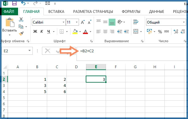
Your formula might not return expected results if the cell’s data type can’t be used in calculations. For example, if you enter a simple formula =2+3 in a cell that’s formatted as text, Excel can’t calculate the data you entered. All you’ll see in the cell is =2+3. To fix this, change the cell’s data type from Text to General like this:

Select the cell.
Select Home and select the arrow to expand the Number or Number Format group (or press Ctrl + 1). Then select General.
Press F2 to put the cell in the edit mode, and then press Enter to accept the formula.

A date you enter in a cell that’s using the Number data type might be shown as a numeric date value instead of a date. To show a number as a date, pick a Date format in the Number Format gallery.

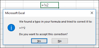
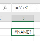
It’s fairly common to use x as the multiplication operator in a formula, but Excel can only accept the asterisk (*) for multiplication. If you use constants in your formula, Excel shows an error message and can fix the formula for you by replacing the x with the asterisk (*).

However, if you use cell references, Excel will return a #NAME? error.

If you create a formula that includes text, enclose the text in quotation marks.

For example, the formula =»Today is » & TEXT(TODAY(),»dddd, mmmm dd») combines the text «Today is » with the results of the TEXT and TODAY functions, and returns say something like Today is Monday, May 30.

In the formula, «Today is » has a space before the ending quotation mark to provide the blank space you want between the words «Today is» and «Monday, May 30.» Without quotation marks around the text, the formula might show the #NAME? error.

You can combine (or nest) up to 64 levels of functions within a formula.

For example, the formula =IF(SQRT(PI())<2,»Less than two!»,»More than two!») has 3 levels of functions; the PI function is nested inside the SQRT function, which in turn is nested inside the IF function.

When you type a reference to values or cells in another worksheet, and the name of that sheet has a non-alphabetical character (such as a space), enclose the name in single quotation marks (‘).

For example, to return the value from cell D3 in a worksheet named Quarterly Data in your workbook, type: =’Quarterly Data’!D3. Without the quotation marks around the sheet name, the formula shows the #NAME? error.

You can also select the values or cells in another sheet to refer to them in your formula. Excel then automatically adds the quotation marks around the sheet names.

When you type a reference to values or cells in another workbook, include the workbook name enclosed in square brackets ([]) followed by the name of the worksheet that has the values or cells.

For example, to refer to cells A1 through A8 on the Sales sheet in the Q2 Operations workbook that’s open in Excel, type: =[Q2 Operations.xlsx]Sales!A1:A8. Without the square brackets, the formula shows the #REF! error.

If the workbook isn’t open in Excel, type the full path to the file.

For example, =ROWS(‘C:My Documents[Q2 Operations.xlsx]Sales’!A1:A8).

Note: If the full path has space characters, enclose the path in single quotation marks (at the beginning of the path and after the name of the worksheet, before the exclamation point).

Tip: The easiest way to get the path to the other workbook is to open the other workbook, then from your original workbook, type =, and use Alt+Tab to shift to the other workbook. Select any cell on the sheet you want, then close the source workbook. Your formula will automatically update to display the full file path and sheet name along with the required syntax. You can even copy and paste the path and use wherever you need it.

Dividing a cell by another cell that has zero (0) or no value results in a #DIV/0! error.

To avoid this error, you can address it directly and test for the existence of the denominator. You could use:

=IF(B1,A1/B1,0)

Which says IF(B1 exists, then divide A1 by B1, otherwise return a 0).

Always check to see if you have any formulas that refer to data in cells, ranges, defined names, worksheets, or workbooks before you delete anything. You can then replace these formulas with their results before you remove the referenced data.

If you can’t replace the formulas with their results, review this information about the errors and possible solutions:

If a formula refers to cells that have been deleted or replaced with other data, and if it returns a #REF! error, select the cell with the #REF! error. In the formula bar, select #REF! and delete it. Then enter the range for the formula again.
If a defined name is missing, and a formula that refers to that name returns a #NAME? error, define a new name that refers to the range you want, or change the formula to refer directly to the range of cells (for example, A2:D8).
If a worksheet is missing, and a formula that refers to it returns a #REF! error, there’s no way to fix this, unfortunately—a worksheet that’s been deleted can’t be recovered.
If a workbook is missing, a formula that refers to it remains intact until you update the formula.

For example, if your formula is =[Book1.xlsx]Sheet1′!A1 and you no longer have Book1.xlsx, the values referenced in that workbook stay available. However, if you edit and save a formula that refers to that workbook, Excel shows the Update Values dialog box and prompts you to enter a file name. Select Cancel, and then make sure this data isn’t lost by replacing the formulas that refer to the missing workbook with the formula results.

Sometimes, when you copy the contents of a cell, you want to paste just the value and not the underlying formula that’s displayed in the formula bar.

For example, you might want to copy the resulting value of a formula to a cell on another worksheet. Or you might want to delete the values that you used in a formula after you copied the resulting value to another cell on the worksheet. Both of these actions cause an invalid cell reference error (#REF!) to appear in the destination cell, because the cells that contain the values you used in the formula can no longer be referenced.

You can avoid this error by pasting the resulting values of formulas, without the formula, in destination cells.

On a worksheet, select the cells that contain the resulting values of a formula that you want to copy.
On the Home tab, in the Clipboard group, select Copy .

Keyboard shortcut: Press CTRL+C.
Select the upper-left cell of the paste area.

Tip: To move or copy a selection to a different worksheet or workbook, select another worksheet tab or switch to another workbook, and then select the upper-left cell of the paste area.
On the Home tab, in the Clipboard group, select Paste , and then select Paste Values, or press Alt > E > S > V > Enter for Windows, or Option > Command > V > V > Enter on a Mac.

To understand how a complex or nested formula calculates the final result, you can evaluate that formula.

Select the formula you want to evaluate.
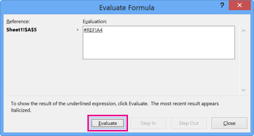
Select Formulas > Evaluate Formula.
Select Evaluate to examine the value of the underlined reference. The result of the evaluation is shown in italics.
If the underlined part of the formula is a reference to another formula, select Step In to show the other formula in the Evaluation box. Select Step Out to go back to the previous cell and formula.

The Step In button isn’t available the second time the reference appears in the formula—or if the formula refers to a cell in another workbook.
Continue until each part of the formula has been evaluated.

The Evaluate Formula tool won’t necessarily tell you why your formula is broken, but it can help point out where. This can be a very handy tool in larger formulas where it might otherwise be difficult to find the problem.
Notes:
- Some parts of the IF and CHOOSE functions won’t be evaluated, and the #N/A error might appear in the Evaluation box.
- Blank references are shown as zero values (0) in the Evaluation box.
- Some functions are recalculated every time the worksheet changes. Those functions, including the RAND, AREAS, INDEX, OFFSET, CELL, INDIRECT, ROWS, COLUMNS, NOW, TODAY, and RANDBETWEEN functions, can cause the Evaluate Formula dialog box to show results that are different from the actual results in the cell on the worksheet.

Need more help?

You can always ask an expert in the Excel Tech Community or get support in the Answers community.

Tip: If you’re a small business owner looking for more information on how to get Microsoft 365 set up, visit Small business help & learning.

FIXED function

This article describes the formula syntax and usage of the FIXED function in Microsoft Excel.

Description

Rounds a number to the specified number of decimals, formats the number in decimal format using a period and commas, and returns the result as text.

Syntax

FIXED(number, [decimals], [no_commas])

The FIXED function syntax has the following arguments:

Number Required. The number you want to round and convert to text.

Decimals Optional. The number of digits to the right of the decimal point.

No_commas Optional. A logical value that, if TRUE, prevents FIXED from including commas in the returned text.

Numbers in Microsoft Excel can never have more than 15 significant digits, but decimals can be as large as 127.

If decimals is negative, number is rounded to the left of the decimal point.

If you omit decimals, it is assumed to be 2.

If no_commas is FALSE or omitted, then the returned text includes commas as usual.

The major difference between formatting a cell containing a number by using a command (On the Home tab, in the Number group, click the arrow next to Number, and then click Number.) and formatting a number directly with the FIXED function is that FIXED converts its result to text. A number formatted with the Cells command is still a number.

Example

Copy the example data in the following table, and paste it in cell A1 of a new Excel worksheet. For formulas to show results, select them, press F2, and then press Enter. If you need to, you can adjust the column widths to see all the data.

Источник

Absolute link in Excel fixes the cell in the formula

Absolute and relative links in Excel

Fill the range of cells A2: A5 with different radii.
In cell B2, enter the formula for calculating the volume of the sphere, which will refer to the value of A2. The formula will look like this: =(4/3)*3.14*A2^3
Copy the formula from B2 along column A2: A5.

As you can see, the relative addresses help to change the address in each formula automatically.

Now instead of numbers we use absolute references:

Use of absolute and relative links in Excel

Fill in the plate, as shown in the picture:

Our new formula should contain at once 2 types of links: absolute and relative.

In C2, enter another formula: = B2 / A $ 2. To change links in Excel, double click on the cell with the left mouse button or press the F2 key on the keyboard.
Copy it to the other cells in the C3:C4 range.

Description of the new formula. The dollar symbol ($) in the address of references fixes the address in the new copied formulas.

Absolute, relative and mixed references in Excel:

$ A $ 2 — address of the absolute reference with fixation on columns and rows, both vertically and horizontally.
$ A2 is a mixed link. When copying a column is fixed, and the row is changed.
A $ 2 is a mixed link. When copying a row is fixed, and the column is changed.

Helpful advice. To avoid entering the dollar symbol ($) manually, after specifying the address, press F4 repeatedly to select the required type: absolute or mixed. It’s fast and convenient.

Источник

How to use the FIXED function in Excel

The FIXED function is a built-in Text function in Microsoft Excel, and its purpose is to format numbers as text with a fixed number of decimals.

How do I create a fixed formula in Excel?

The formula for the FIXED function is Fixed (number, [decimal], [no_commas] . The syntax for the FIXED function is below:

Number: The number you want to round and convert to text. It is required.
Decimals: The number of digits to the right of the decimal point. It is optional.
No_commas: A logical value that, if TRUE, prevents FIXED from including commas in the returned text. It is optional.

How to use the FIXED function in Excel

Follow the steps below to use the FIXED function in Excel:

Launch Microsoft Excel
Create a table or use an existing table from your files
Place the formula into the cell you want to see the result
Press the Enter Key

Launch Microsoft Excel.

Create a table or use an existing table from your files.

Type the formula into the cell you want to place the result =FIXED(A2,1).

Then press the Enter key to see the result.

You will notice that Excel will round the number one digit to the right of the decimal point.

If you choose to type the formula as FiXED(A2,-1), Excel will round the number as one digit to the left of the decimal point. Result 530.

If you choose to type the formula as =FIXED(A2,1, TRUE), Excel will round the numbers round the number one digit to the right of the decimal point. Result 534.6.

If you choose to type the formula as =FIXED(A2,-1, TRUE), Excel will round the number as one digit to the left of the decimal point, without commas. Result 530.

If you type the formula as =FIXED(A2), Excel will round the number two digits to the left of the decimal point. Result 534.56.

There are two other methods to use the FIXED function.

1] Click the fx button on the top left of the Excel worksheet.

An Insert Function dialog box will appear.

Inside the dialog box in the section, Select a Category, select TEXT from the list box.

In the section Select a Function, choose the FIXED function from the list.

A Function Arguments dialog box will open.

In the Number entry box, input into the entry box cell A2.

In the Decimal entry box, input into box 1. The Decimal argument is optional

2] Click the Formulas tab, click the Text button in the Function Library group.

Then select FIXED from the drop-down menu.

A Function Arguments dialog box will open.

How do I copy a fixed formula in Excel?

In Microsoft Excel, you can copy any formula by copying the cell to which it is applied. If you want to copy the FIXED formula, select the cell in which the FIXED formula is applied and press the Ctrl + C keys. The formula is now copied. After that, select the cell to which you want to apply this formula and paste it by pressing the Ctrl + V keys. Excel will automatically correct the FIXED formula and display the correct result.

We hope this tutorial helps you understand how to use the FIXED function in Microsoft Excel; if you have questions about the tutorial, let us know in the comments.

Источник

How to Fix Excel Formulas that are Not Calculating or Updating

Bottom Line: Learn about the different calculation modes in Excel and what to do if your formulas are not calculating when you edit dependent cells.

Skill Level: Beginner

Watch the Tutorial

Download the Excel File

You can follow along using the same workbook I use in the video. I’ve attached it below:

Loan Amortization Schedule – Manual Calc Example.xlsx

Why Aren’t My Formulas Calculating?

If you’ve ever been in a situation where the formulas in your spreadsheet are not automatically calculating as they should, you know how frustrating it can be.

This was happening to my friend Brett. He was telling me that he was working with a file and it wasn’t recalculating the formulas as he was entering data. He found that he had to edit each cell and hit Enter for the formula in the cell to update.

And it was only happening on his computer at home. His work computer was working just fine. This was driving him crazy and wasting a lot of time.

The most likely cause of this issue is the Calculation Option mode, and it’s a critical setting that every Excel user should know about.

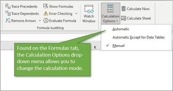
To check what calculation mode Excel is in, go to the Formulas tab, and click on Calculation Options. This will bring up a menu with three choices. The current mode will have a checkmark next to it. In the image below, you can see that Excel is in Manual Calculation Mode.

When Excel is in Manual Calculation mode, the formulas in your worksheet will not calculate automatically. You can quickly and easily fix your problem by changing the mode to Automatic. There are cases when you might want to use Manual Calc mode, and I explain more about that below.

Calculation Settings are Confusing!

It’s really important to know how the calculation mode can change. Technically, it’s is an application-level setting. That means that the setting will apply to all workbooks you have open on your computer.

As I mention in the video above, this was the issue with my friend Brett. Excel was in Manual calculation mode on his home computer and his files weren’t calculating. When he opened the same files on his work computer, they were calculating just fine because Excel was in Automatic calculation mode on that computer.

However, there is one major nuance here. The workbook (Excel file) also stores the last saved calculation setting and can change/override the application-level setting.

This should only happen for the first file you open during an Excel session.

For example, if you change Excel to manual calc mode before you save & close the file, then that setting is stored with the workbook. If you then open that workbook as the first workbook in your Excel session, the calculation mode will be changed to manual.

All subsequent workbooks that you open during that session will also be in manual calculation mode. If you save and close those files, the manual calc mode will be stored with the files as well.

The confusing part about this behavior is that it only happens for the first file you open in a session. Once you close the Excel application completely and then re-open it, Excel will return to automatic calculation mode if you start by opening a new blank file or any file that is in automatic calculation mode.

Therefore, the calculation mode of the first file you open in an Excel session dictates the calculation mode for all files opened in that session. If you change the calculation mode in one file, it will be changed for all open files.

Note: I misspoke about this in the video when I said that the calculation setting doesn’t travel with the workbook, and I will update the video.

The 3 Calculation Options

There are three calculation options in Excel.

Automatic Calculation means that Excel will recalculate all dependent formulas when a cell value or formula is changed.

Manual Calculation means that Excel will only recalculate when you force it to. This can be with a button press or keyboard shortcut. You can also recalculate a single cell by editing the cell and pressing Enter.

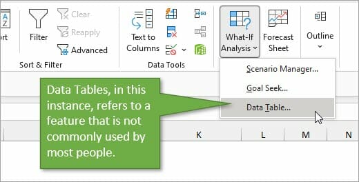
Automatic Except for Data Tables means that Excel will recalculate automatically for all cells except those that are used in Data Tables. This is not referring to normal Excel Tables that you might work with frequently. This refers to a scenario-analysis tool that not many people use. You find it on the Data tab, under the What-If Scenarios button. So unless you’re working with those Data Tables, it’s unlikely you will ever purposely change the setting to that option.

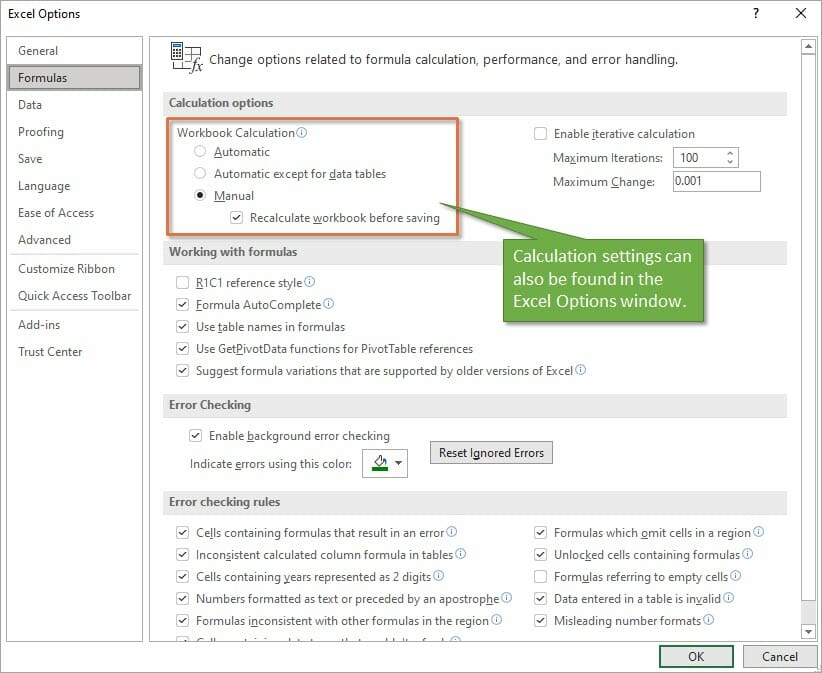
In addition to finding the Calculation setting on the Data tab, you can also find it on the Excel Options menu. Go to File, then Options, then Formulas to see the same setting options in the Excel Options window.

Under the Manual Option, you’ll see a checkbox for recalculating the workbook before saving, which is the default setting. That’s a good thing because you want your data to calculate correctly before you save the file and share it with your co-workers.

Click to enlarge

Why Would I Use Manual Calculation Mode?

If you are wondering why anyone would ever want to change the calculation from Automatic to Manual, there’s one major reason. When working with large files that are slow to calculate, the constant recalculation whenever changes are made can sometimes slow your system. Therefore people will sometimes switch to Manual mode while working through changes on worksheets that have a lot of data, and then will switch back.

When you are in Manual Calculation mode, you can force a calculation at any time using the Calculate Now button on the Formulas tab.

The keyboard shortcut for Calculate Now is F9 , and it will calculate the entire workbook. If you want to calculate just the current worksheet, you can choose the button below it: Calculate Sheet. The keyboard shortcut for that choice is Shift + F9 .

Here is a list of all Recalculate keyboard shortcuts:

Shortcut	Description
F9	Recalculate formulas that have changed since the last calculation, and formulas dependent on them, in all open workbooks. If a workbook is set for automatic recalculation, you do not need to press F9 for recalculation.
Shift+F9	Recalculate formulas that have changed since the last calculation, and formulas dependent on them, in the active worksheet.
Ctrl+Alt+F9	Recalculate all formulas in all open workbooks, regardless of whether they have changed since the last recalculation.
Ctrl+Shift+Alt+F9	Check dependent formulas, and then recalculate all formulas in all open workbooks, regardless of whether they have changed since the last recalculation.

Source: Microsoft: Change formula recalculation article

Macro Changing to Manual Calculation Mode

If you find that your workbook is not automatically calculating, but you didn’t purposely change the mode, another reason that it may have changed is because of a macro.

Now I want to preface this by saying that the issue is NOT caused by all macros. It’s a specific line of code that a developer might use to help the macro run faster.

The following line of VBA code tells Excel to change to Manual Calculation mode.

Sometimes the author of the macro will add that line at the beginning so that Excel does not attempt to calculate while the macro runs. The setting should then changed be changed back at the end of the macro with the following line.

This technique can work well for large workbooks that are slow to calculate.

However, the problem arises when the macro doesn’t get to finish—perhaps due to an error, program crash, or unexpected system issue. The macro changes the setting to Manual and it doesn’t get changed back.

As I mention in the video, this was exactly what happened to my friend Brett, and he was NOT aware of it. He was left in manual calc mode and didn’t know why, or how to get Excel calculating again.

Therefore, if you are using this technique with your macros, I encourage you to think about ways to mitigate this issue. And also warn your users of the potential of Excel being left in manual calc mode.

I also recommend NOT changing the Calculation property with code unless you absolutely need to. This will help prevent frustration and errors for the users of your macros.

Conclusion

I hope this information is helpful for you, especially if you are currently dealing with this particular issue. If you have any questions or comments about calculation modes, please share them in the comments.

Источник

Часто так бывает, что при копировании формул, Вам нужно, что бы ссылка на ячейку в формуле осталась такой же, как и была, а не переместилась относительно исходного места. Тогда Вам на помощь придет такая функция в Excel, как фиксация ссылок на ячейки в Экселе. Остановимся подробно на всех вариантах.

1. Способ, как закрепить (зафиксировать) строку и столбец в формуле Excel

Для того, что бы ссылка на ячейку не изменялась полностью, т.е. адрес столбца и строки оставались неизменными, проделайте следующие простые действия:

Кликните на ячейке с формулой.
Кликните в строке формул на адрес той ячейке, что Вы хотите закрепить.
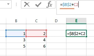
Нажмите F4 один раз.

В результате ссылка на ячейку должна быть дополнена знаками доллара, к примеру у Вас в формуле была ссылка на ячейку B2, то после вышеуказанной операции, ссылка на ячейку должна стать $B$2.

Разберем подробно, что значит знак доллара перед буквой и перед числом:

Знак доллара перед буквой означает, что при перемещении формулы вправо или влево, т.е. смещая ее по столбцам, ссылка на столбец ячейки в формуле меняться не будет.
Знак доллара перед числом означает, что при перемещении формулы вверх
или вниз, т.е. смещая ее по строкам, ссылка на строку ячейки в
формуле меняться не будет.

2. Способ, как закрепить (зафиксировать) строку в формуле Excel

Способ полностью аналогичный тому, что описан выше, только Вам нужно будет нажать дважды на F4. К примеру, если у Вас в формуле ссылка на ячейку B2, то Вы получите B$2. Это значит, что теперь при перемещении формулы, будет изменяться буква столбца, а номер строки будет оставаться неизменным.

3. Способ, как закрепить (зафиксировать) столбец в формуле Excel

Все тоже самое, что и в вариантах выше, только нажмите на клавишу F4 трижды. Вы должны получить ссылку на ячейку вида $B2, т.е. теперь при перемещении формулы, будет меняться номер строки, а буква столбца будет неизменной.

4. Способ, как отменить фиксацию ячейки в формуле Excel

В случае если Вам наоборот нужно отменить фиксацию ячейки в формуле, то нажмите F4 несколько раз, так что бы в ссылке на ячейку не осталось знаков $, тогда при перемещении формулы, будет изменяться адрес ячейки как по строкам, так и по столбцам.

Спасибо за внимание. Остались вопросы — задавайте их в комментариях к статье. Подписывайтесь на наши группы Вконтакте, Facebook, Twitter, Google+ и будете получать первыми информацию о новых статьях на сайте.

Источник

Absolute and relative links in Excel

Use of absolute and relative links in Excel

Need more help?

See Also

Need more help?

Want more options?

FIXED function

Description

Syntax

Example

Absolute link in Excel fixes the cell in the formula

Absolute and relative links in Excel

Use of absolute and relative links in Excel

How to use the FIXED function in Excel

How do I create a fixed formula in Excel?

How to use the FIXED function in Excel

How do I copy a fixed formula in Excel?

How to Fix Excel Formulas that are Not Calculating or Updating

Watch the Tutorial

Download the Excel File

Why Aren’t My Formulas Calculating?

Calculation Settings are Confusing!

The 3 Calculation Options

Why Would I Use Manual Calculation Mode?

Macro Changing to Manual Calculation Mode

Conclusion

1. Способ, как закрепить (зафиксировать) строку и столбец в формуле Excel

2. Способ, как закрепить (зафиксировать) строку в формуле Excel

3. Способ, как закрепить (зафиксировать) столбец в формуле Excel

4. Способ, как отменить фиксацию ячейки в формуле Excel